จำลองการกระเจิงนิวตรอนในวัสดุควอนตัมด้วยวงจรควอนตัม

ประมาณการการใช้งาน: 13 นาทีบนโปรเซสเซอร์ Heron r2 (หมายเหตุ: นี่เป็นเพียงการประมาณการเท่านั้น เวลาการรันจริงของคุณอาจแตกต่างกัน)

ควรใช้บทช่วยสอนใด?

ใช้บทช่วยสอนนี้เพื่อเรียนรู้การนำไปใช้งานทีละขั้นตอน โดยการคำนวณแบบคลาสสิกรันในเครื่องท้องถิ่นบนแล็ปท็อปของคุณ และการรันบนฮาร์ดแวร์บน QPU ของ IBM Quantum® ตัวอย่างขนาดใหญ่ต้องการหน่วยความจำจำนวนมาก และการคอมไพล์ควอนตัมแบบประมาณ (approximate quantum compiling หรือ AQC) อาจใช้เวลาหลายชั่วโมงบนทรัพยากรแล็ปท็อปทั่วไป หากต้องการถ่ายโอนการบีบอัดไปยังทรัพยากรการประมวลผลและหน่วยความจำของ Qiskit Serverless ให้ใช้ บทช่วยสอนคู่กันบน Serverless

ผลลัพธ์การเรียนรู้

• สเปกตรัม inelastic neutron scattering (INS) เชื่อมโยงกับ dynamical structure factor (DSF) ของโมเดล spin ควอนตัมอย่างไร

• วิธีเตรียม ground state, ใช้ local perturbation และทำ Trotter time evolution บนวงจรควอนตัม

• วิธีใช้ approximate quantum compiling (AQC) ด้วย qiskit-addon-aqc-tensor เพื่อบีบอัดวงจร Trotter ที่ลึกสำหรับการ execute บนฮาร์ดแวร์

• วิธีดึง retarded Green's function (RGF) จากค่าคาดหวังของ qubit และแปลงฟูริเยร์ให้เป็น DSF

ข้อกำหนดเบื้องต้น

• พื้นฐานของข้อมูลควอนตัม

• การออกแบบอัลกอริทึมแบบ variational

• แนะนำ Qiskit primitives (Estimator และ Sampler)

ความเป็นมา

ใน tutorial นี้ เราจะทำซ้ำผลลัพธ์ของ Lee et al., arXiv:2603.15608

การกระเจิงนิวตรอนช่วยให้นักวิจัยวัดคุณลักษณะของวัสดุที่เกี่ยวข้องกับความยั่งยืน รวมถึงขั้วไฟฟ้าแบตเตอรี่ บทเรียนนี้สำรวจว่าวงจรควอนตัมสามารถจำลองการกระตุ้นทางแม่เหล็ก (magnetic excitation) และเชื่อมโยงโมเดลเชิงทฤษฎีเข้ากับการวัดการกระเจิงได้อย่างไร ตัวอย่าง quantum-magnet ของบทเรียนนี้พัฒนาวิธีการสำหรับศึกษาพฤติกรรมของวัสดุ ซึ่งมีส่วนช่วยเครื่องมือวิจัยที่กว้างขึ้นสำหรับการค้นพบวัสดุ

Inelastic neutron scattering และ dynamical structure factor

Inelastic neutron scattering (INS) เป็นหนึ่งในเครื่องมือทดลองที่ทรงพลังที่สุดในการตรวจสอบ excitation ของแม่เหล็กในวัสดุควอนตัม เมื่อลำนิวตรอนความร้อนหรือเย็นกระทบกับผลึก นิวตรอนแต่ละตัวจะแลกเปลี่ยนทั้ง momentum $\mathbf{q}$ และพลังงาน $\omega$ กับระบบย่อยแม่เหล็ก ความเข้มของการกระเจิงที่วัดได้จะแปรผันตาม dynamical structure factor (DSF)

$S^{\alpha\beta}(q,\omega) = \sum_{j} e^{-iq\,j}\int_{-\infty}^{\infty} dt\; e^{i\omega t}\, \langle S_0^{\alpha}(0)\, S_j^{\beta}(t)\rangle,$

ซึ่งเข้ารหัสความสัมพันธ์เชิงพื้นที่-เวลาแบบเต็มของ degree of freedom ของ spin

KCuF$_3$: แม่เหล็ก Luttinger-liquid ต้นแบบ

โพแทสเซียมคอปเปอร์ฟลูออไรด์ (KCuF$_3$) เป็นสาร antiferromagnet แบบ quasi-one-dimensional ที่ chain ของไอออน spin-$\frac{1}{2}$ Cu$^{2+}$ มีปฏิสัมพันธ์กันผ่าน nearest-neighbor Heisenberg exchange $J$ ในขณะที่ interchain coupling มีเพียง $\sim 2.7\%$ ของ $J$ ที่ $T = 6\;\mathrm{K}$ ซึ่งมีข้อมูล INS อยู่ สเปกตรัมถูกครอบงำด้วย spinon excitation แบบ fractionalized ที่เป็นลักษณะเฉพาะของ Tomonaga-Luttinger liquid เนื่องจาก dynamics ภายใน chain ถูกอธิบายอย่างดีด้วย Hamiltonian แบบ one-dimensional spin-$\frac{1}{2}$ XXZ ที่จุด isotropic ($\epsilon = 1$)

$H = J\sum_{i}\left[S_i^Z S_{i+1}^Z + \epsilon\left(S_i^X S_{i+1}^X + S_i^Y S_{i+1}^Y\right)\right],$

KCuF$_3$ ทำหน้าที่เป็น benchmark ที่เหมาะสำหรับการจำลองควอนตัม: Hamiltonian นั้นง่ายพอที่จะ implement บนโปรเซสเซอร์ควอนตัม แต่ ground state มี entanglement สูงและสเปกตรัม excitation มี two-spinon continuum ที่กว้าง

หมายเหตุ: tutorial นี้กำหนด $J = 1$ เป็นหน่วยพลังงานและใช้การ normalize $H = J\sum_i[\ldots]$ ซึ่งสอดคล้องกับ Hamiltonian ท้องถิ่น $H_\mathrm{loc} = J(S^X S^X + S^Y S^Y + S^Z S^Z)$ ที่ใช้ใน implementation วงจรของงานวิจัย (Fig. S3 ของภาคผนวก) Hamiltonian แบบเต็มของงานวิจัย (Eq. 3) มีตัวประกอบเพิ่มเติมโดยรวมเป็น 2 ดังนั้น $J$ ของงานวิจัยจึงเป็นสองเท่าของ $J$ ที่ใช้ที่นี่

สิ่งที่เราจำลองและวัด

ปริมาณทางฟิสิกส์ที่เราคำนวณคือ retarded Green's function (RGF) ที่นิยามเป็นฟังก์ชันสหสัมพันธ์ spin-spin ที่ขึ้นกับเวลา

$G^R_{\alpha,\beta}(j, j_c, t) = -\frac{i}{2}\,\langle\psi_{\mathrm{GS}}|\,S_j^\alpha(t)\,S_{j_c}^\beta(0) - S_{j_c}^\beta(0)\,S_j^\alpha(t)\,|\psi_{\mathrm{GS}}\rangle,$

โดยที่ $j_c$ เป็น site อ้างอิง (จุดศูนย์กลางของ chain) และ $S_j^\alpha(t) = e^{iHt}S_j^\alpha e^{-iHt}$ เป็น spin operator ในภาพ Heisenberg ใน tutorial นี้เราจะเน้นที่ส่วนประกอบ $zz$ ($\alpha = \beta = z$) บนคอมพิวเตอร์ควอนตัม RGF จะถูกเข้าถึงโดยการเตรียม ground state, ใช้ local perturbation ที่ $j_c$, ทำ time-evolve ของ state ที่ถูก perturb และวัดค่าคาดหวังของ single-qubit $\langle\sigma_j^z\rangle$ ที่ทุก site $j$ สำหรับแต่ละ time step ข้อมูลเชิงลึกที่สำคัญคือแต่ละ $\langle\sigma_j^z\rangle$ ให้ความแตกต่างจาก magnetization ของ ground state เนื่องจาก isotropic Heisenberg antiferromagnet มี magnetization สุทธิต่อ site เป็นศูนย์ ($\langle\sigma_j^z\rangle_\mathrm{GS} = 0$) ค่าที่วัดได้ดิบจึงให้ $G^R(j, j_c, t)$ โดยตรงโดยไม่ต้องหักลบใดๆ อย่างชัดเจน

โดยการเก็บรวบรวม $G^R(j, j_c, t)$ ทั่วทุก site และ time step เราจะประกอบเป็นชุดข้อมูลสองมิติ ซึ่งจะถูกแปลงฟูริเยร์ทั้งในเชิงพื้นที่และเวลาเพื่อสร้าง dynamical structure factor $S(q,\omega)$ DSF เป็นปริมาณที่วัดได้โดยตรงในการทดลอง INS: มันบอกเราว่า excitation ของแม่เหล็กใดมีอยู่ที่ momentum $q$ และพลังงาน $\omega$ แต่ละคู่ สำหรับ isotropic Heisenberg chain สเปกตรัม excitation ที่แม่นตรง (exact) คือ two-spinon continuum ซึ่งเป็นแถบกว้างของความเข้มการกระเจิงที่รูปร่างของมันทำหน้าที่เป็น benchmark แบบ end-to-end ที่เข้มงวดสำหรับการจำลองควอนตัม: มันตรวจสอบความถูกต้องของการเตรียม ground state, perturbation, Trotter time evolution และ protocol การวัดทั้งหมดพร้อมกัน

Workflow การจำลองควอนตัม

workflow สะท้อนฟิสิกส์ของเหตุการณ์ INS เรา (1) เตรียม ground state แบบ many-body $|\psi_{\mathrm{GS}}\rangle$ บน $n$ qubit (2) ใช้ local spin-flip perturbation $U_{j_c} = \frac{1}{\sqrt{2}}(I - i\sigma^z_{j_c})$ ที่จุดศูนย์กลางของ chain เพื่อจำลองการถ่ายโอน spin ของนิวตรอน (3) ทำการวิวัฒนาการภายใต้ $H$ สำหรับ time step แบบไม่ต่อเนื่องโดยใช้ Trotterization อันดับสอง และ (4) วัด $\langle\sigma_i^z\rangle$ บนทุก qubit ในแต่ละ step เพื่อได้ RGF การแปลงฟูริเยร์แบบไม่ต่อเนื่องสองมิติจึงให้ DSF $S(q,\omega)$

observable ที่เราวัดในทุก time step คือ $\sigma_i^z$ บนแต่ละ qubit $i$ ใน Qiskit สิ่งนี้ถูกแสดงเป็นรายการของ operator SparsePauliOp: single-qubit $Z$ หนึ่งตัวฝังอยู่ใน identity string ของ $n$-qubit สำหรับแต่ละ site observable เหล่านี้ถูกสร้างขึ้นเพียงครั้งเดียวต่อ instance ของปัญหาในระหว่างขั้นตอนการแม็ปปัญหา (Step 1) และนำกลับมาใช้ซ้ำสำหรับทุกวงจรที่ scale นั้น

การคอมไพล์เชิงควอนตัมโดยประมาณ (Approximate quantum compiling, AQC)

วงจร Trotter ที่ลึกสามารถถูกบีบอัดด้วย approximate quantum compiling (AQC) ซึ่งแทนที่ชั้น Trotter แรกๆ หลายชั้นด้วย ansatz แบบมีพารามิเตอร์ที่สั้นกว่า โดยพารามิเตอร์ของมันถูก optimize แบบคลาสสิกเพื่อ maximize fidelity ระดับ MPS กับวงจรลึกต้นฉบับ Trotter step ที่เหลือจะถูกต่อเข้าไปแบบ exact (ไม่ผ่านการประมาณ) ทำให้ได้วงจร "AQC + Trotter" แบบผสมที่มี two-qubit gate น้อยลงอย่างมาก

การจำลองด้วย MPS

สำหรับระบบ one-dimensional วิธี matrix-product-state (MPS) สามารถจำลองทั้งการเตรียม ground state (ด้วย density matrix renormalization group หรือ DMRG) และการวิวัฒนาการตามเวลาระดับวงจรได้อย่างมีประสิทธิภาพ โดยการควบคุม bond dimension $\chi$ เราแลกความแม่นยำกับต้นทุนการคำนวณ ใน tutorial นี้เราใช้การจำลองด้วย MPS ภายใน qiskit-addon-aqc-tensor เพื่อคำนวณ AQC ansätze ที่มี fidelity สูงซึ่งบีบอัดวงจร Trotter ที่ลึกสำหรับการ execute บนฮาร์ดแวร์

ข้อกำหนด

ก่อนเริ่ม tutorial นี้ ตรวจสอบให้แน่ใจว่าคุณได้ติดตั้งสิ่งต่อไปนี้แล้ว:

• Qiskit SDK พร้อมการรองรับ visualization

• Qiskit Runtime (pip install qiskit-ibm-runtime)

• qiskit-addon-aqc-tensor พร้อม extras ของ quimb และ JAX (pip install 'qiskit-addon-aqc-tensor[quimb-jax]')

การตั้งค่า

# Added by doQumentation — installs the packages this notebook needs if they are missing
import importlib.util

_needed = {"matplotlib": "matplotlib", "numpy": "numpy", "qiskit": "qiskit", "qiskit_addon_aqc_tensor": "qiskit-addon-aqc-tensor", "qiskit_ibm_runtime": "qiskit-ibm-runtime", "qiskit_quimb": "qiskit-quimb", "quimb": "quimb", "scipy": "scipy"}
_missing = [pip for module, pip in _needed.items()
            if importlib.util.find_spec(module) is None]
# One at a time, so a package that fails to install does not block the others
for _pip in _missing:
    %pip install -q {_pip}
if not _missing:
    print("\u2713 All required packages are installed")

import timeit
import warnings
from collections.abc import Iterator, Sequence
from functools import partial

import matplotlib.pyplot as plt
import numpy as np
import quimb.tensor as qtn
import scipy.optimize
from numpy.typing import NDArray
from qiskit import QuantumCircuit
from qiskit.circuit import CircuitInstruction, ParameterVector, Qubit
from qiskit.circuit.library import PauliEvolutionGate
from qiskit.primitives import StatevectorEstimator
from qiskit.quantum_info import SparsePauliOp
from qiskit.transpiler.preset_passmanagers import generate_preset_pass_manager
from qiskit_addon_aqc_tensor import generate_ansatz_from_circuit
from qiskit_addon_aqc_tensor.objective import MaximizeStateFidelity
from qiskit_addon_aqc_tensor.simulation import tensornetwork_from_circuit
from qiskit_addon_aqc_tensor.simulation.quimb import QuimbSimulator
from qiskit_ibm_runtime import EstimatorV2 as Estimator
from qiskit_ibm_runtime import QiskitRuntimeService
from qiskit_quimb import quimb_circuit
from scipy.sparse import SparseEfficiencyWarning

# scipy.sparse.linalg.expm (reached via PauliEvolutionGate.to_matrix) prefers
# CSC and warns when handed the CSR matrix from SparsePauliOp.to_matrix; the
# result is unaffected, so silence the cosmetic warning.
warnings.filterwarnings("ignore", category=SparseEfficiencyWarning)

def xxz_hamiltonian_mpo(
    n_qubits: int, interaction: float = 1.0, anisotropy: float = 1.0
) -> qtn.MatrixProductOperator:
    """1D XXZ Hamiltonian as a quimb MPO.

    Builds the Hamiltonian using ``qtn.SpinHam1D``.

    Args:
        n_qubits: Number of sites.
        interaction: Overall interaction strength (J in the paper).
        anisotropy: XY/Z anisotropy (ε in the paper). ``ε = 1`` is the
            isotropic Heisenberg point; ``ε = 0`` is the Ising limit.

    Returns:
        The Hamiltonian as a matrix product operator.
    """
    builder = qtn.SpinHam1D(S=1 / 2)
    builder += interaction * anisotropy * 0.5, "+", "-"
    builder += interaction * anisotropy * 0.5, "-", "+"
    builder += interaction, "Z", "Z"
    return builder.build_mpo(L=n_qubits)

def build_ground_state_ansatz(n_qubits: int, n_layers: int) -> QuantumCircuit:
    """Hamiltonian variational ansatz (HVA) circuit for ground-state preparation.

    Starts from a product of singlet pairs and applies alternating
    odd/even layers of parameterized XXZ pair-evolution gates.

    The returned circuit is parameterized: it carries a ``ParameterVector``
    named ``"theta"`` of length ``2 * n_layers`` whose values must be
    assigned (e.g. via ``circuit.assign_parameters``) before simulation.
    Element ``2 * r`` is the odd-layer angle and element ``2 * r + 1`` is the
    even-layer angle of layer ``r``.

    Args:
        n_qubits: Number of qubits (must be even).
        n_layers: Number of HVA layers.

    Returns:
        The parameterized HVA preparation circuit.
    """
    theta = ParameterVector("theta", 2 * n_layers)
    circuit = QuantumCircuit(n_qubits)
    # Initial singlet product state
    for i in range(n_qubits // 2):
        circuit.x(2 * i)
        circuit.x(2 * i + 1)
        circuit.h(2 * i + 1)
        circuit.cx(2 * i + 1, 2 * i)
    # Variational layers: each pair gate is exp(-i theta (XX+YY+ZZ)/2)
    pair_ham = SparsePauliOp(
        ["XX", "YY", "ZZ"], coeffs=[0.5, 0.5, 0.5]
    )  # H_pair (HVA form)
    for r in range(n_layers):
        for i in range(1, (n_qubits + 1) // 2):  # odd layer
            circuit.append(
                PauliEvolutionGate(pair_ham, time=theta[2 * r]),
                [2 * i - 1, 2 * i],
            )
        for i in range(n_qubits // 2):  # even layer
            circuit.append(
                PauliEvolutionGate(pair_ham, time=theta[2 * r + 1]),
                [2 * i, 2 * i + 1],
            )
    return circuit

def optimize_ground_state_ansatz(
    ansatz: QuantumCircuit,
    x0: NDArray[np.floating],
    target_mps: qtn.MatrixProductState,
    *,
    max_bond: int | None = None,
    cutoff: float = 1e-10,
    method: str = "COBYQA",
    options: dict | None = None,
) -> scipy.optimize.OptimizeResult:
    """Optimize HVA parameters by maximizing fidelity with a target MPS.

    The HVA circuit is simulated as a matrix product state with the given
    bond-dimension truncation, and the parameters are optimized to maximize
    the state fidelity ``|<psi_HVA | target_mps>|**2`` with the DMRG ground
    state. Both states are normalized, so the minimized objective is the
    infidelity ``1 - |<psi_HVA | target_mps>|**2``.

    Args:
        ansatz: Parameterized HVA circuit from ``build_ground_state_ansatz``.
            The length of ``x0`` must equal ``ansatz.num_parameters``.
        x0: Initial parameters.
        target_mps: Target MPS (DMRG ground state) to maximize fidelity with.
        max_bond: Maximum MPS bond dimension during gate application.
        cutoff: Singular-value cutoff during gate application.
        method: ``scipy.optimize.minimize`` method.
        options: Options dict forwarded to ``scipy.optimize.minimize``.

    Returns:
        The Scipy OptimizeResult.
    """

    def infidelity(params: NDArray[np.floating]) -> float:
        circuit = ansatz.assign_parameters(params)
        circuit_mps = quimb_circuit(
            circuit.decompose(["PauliEvolution"]),
            quimb_circuit_class=qtn.CircuitMPS,
            max_bond=max_bond,
            cutoff=cutoff,
        )
        return 1 - abs(circuit_mps.psi.H @ target_mps) ** 2

    return scipy.optimize.minimize(
        infidelity, np.asarray(x0), method=method, options=options
    )

def trotter_evolution(
    qubits: Sequence[Qubit],
    interaction: float,
    anisotropy: float,
    time_step: float,
    n_steps: int,
) -> Iterator[CircuitInstruction]:
    """Second-order Trotter steps of the XXZ pair Hamiltonian.

    While the paper used a hand-optimized circuit for the Trotter steps, we use
    PauliEvolutionGate here for simplicity and generality. The final two-qubit gate
    count and gate depth are equivalent when transpiled with ``optimization_level=3``.

    Args:
        qubits: Qubits to act on (length ``n_qubits``).
        interaction: Overall interaction strength (J in the paper).
        anisotropy: XY/Z anisotropy (ε in the paper). ``ε = 1`` is the
            isotropic Heisenberg point; ``ε = 0`` is the Ising limit.
        time_step: Per-step Trotter time.
        n_steps: Number of Trotter steps.

    Yields:
        ``CircuitInstruction``s implementing the Trotter steps.
    """
    if n_steps == 0:
        return
    n_qubits = len(qubits)
    pair_ham = SparsePauliOp(
        ["XX", "YY", "ZZ"],
        coeffs=[
            0.25 * interaction * anisotropy,
            0.25 * interaction * anisotropy,
            0.25 * interaction,
        ],
    )
    half_evo = PauliEvolutionGate(pair_ham, time=time_step / 2)
    full_evo = PauliEvolutionGate(pair_ham, time=time_step)
    for i in range(n_qubits // 2):  # half even layer
        yield CircuitInstruction(half_evo, (qubits[2 * i], qubits[2 * i + 1]))
    for i in range(n_qubits // 2 - 1):  # full odd layer
        yield CircuitInstruction(
            full_evo, (qubits[2 * i + 1], qubits[2 * i + 2])
        )
    for _ in range(n_steps - 1):  # interior steps
        for i in range(n_qubits // 2):
            yield CircuitInstruction(
                full_evo, (qubits[2 * i], qubits[2 * i + 1])
            )
        for i in range(n_qubits // 2 - 1):
            yield CircuitInstruction(
                full_evo, (qubits[2 * i + 1], qubits[2 * i + 2])
            )
    for i in range(n_qubits // 2):  # half even layer
        yield CircuitInstruction(half_evo, (qubits[2 * i], qubits[2 * i + 1]))

def get_dsf(
    n_qubits: int,
    rgf_mat: NDArray[np.floating],
    time_step: float,
    n_steps: int,
    n_points_momentum: int,
    n_points_frequency: int,
) -> NDArray[np.floating]:
    """Compute the dynamical structure factor from the retarded Green's function.

    Uses the center-site approximation and a discrete Fourier transform.
    The result is symmetrized about the momentum axis and clipped to
    non-negative values, ready for plotting.

    Args:
        n_qubits: Number of qubits (sites).
        rgf_mat: RGF matrix of shape ``(n_steps, n_qubits)``.
        time_step: Trotter time-step size.
        n_steps: Number of time steps.
        n_points_momentum: Number of momentum points.
        n_points_frequency: Number of frequency points.

    Returns:
        DSF array of shape ``(n_points_frequency, n_points_momentum)``,
        symmetrized about the momentum axis and clipped to non-negative values.
    """
    max_frequency = np.pi / time_step
    momentum_range = np.linspace(0, 2 * np.pi, n_points_momentum)
    frequency_range = np.linspace(0, max_frequency, n_points_frequency)
    result = np.zeros((frequency_range.shape[0], momentum_range.shape[0]))
    center = n_qubits // 2 - 1
    for iw, w in enumerate(frequency_range):
        exponent = np.exp(1j * w * time_step * np.arange(1, n_steps + 1))
        # S = sigma/2, so two spin operators contribute a factor of (1/2)(1/2) = 1/4.
        rgf_omega = (
            np.dot(rgf_mat.T, exponent) * time_step / 4
        )  # S(omega): time Fourier slice of the Green's function
        for iq, q in enumerate(momentum_range):
            momentum_phases = np.exp(
                -1j * q * np.arange(-center, center + 2, 1)
            )
            result[iw, iq] = np.imag(np.dot(rgf_omega, momentum_phases))
    result = -(result + result[:, ::-1]) / 2
    result = np.clip(result, a_min=0, a_max=None)
    return result

def plot_dsf(
    dsf: NDArray[np.floating],
    time_step: float,
    n_points_momentum: int,
    n_points_frequency: int,
    title: str | None = None,
) -> None:
    """Heat-map of the dynamical structure factor.

    Args:
        dsf: DSF array of shape ``(n_points_frequency, n_points_momentum)``.
        time_step: Trotter time-step size.
        n_points_momentum: Number of momentum points.
        n_points_frequency: Number of frequency points.
        title: Optional plot title.
    """
    max_frequency = np.pi / time_step
    momentum_range = np.linspace(0, 2 * np.pi, n_points_momentum)
    frequency_range = np.linspace(0, max_frequency, n_points_frequency)
    x, y = np.meshgrid(momentum_range, frequency_range)
    fig, ax = plt.subplots(figsize=(8, 5))
    c = ax.pcolormesh(x, y, dsf / np.max(dsf), cmap="viridis", shading="auto")
    fig.colorbar(c, ax=ax, label="Normalized intensity")
    ax.set_ylim(0, 3.6)
    ax.set_xlim(0, 2 * np.pi)
    ax.set_xlabel(r"$q$", fontsize=16)
    ax.set_ylabel(r"$\tilde{\omega} = \omega / J$", fontsize=16)
    ax.set_xticks([0, np.pi / 2, np.pi, 3 * np.pi / 2, 2 * np.pi])
    ax.set_xticklabels(["0", r"$\pi/2$", r"$\pi$", r"$3\pi/2$", r"$2\pi$"])
    if title:
        ax.set_title(title, fontsize=14)
    plt.tight_layout()
    plt.show()

def plot_rgf(
    n_qubits: int,
    rgf_mat: NDArray[np.floating],
    time_step: float,
    n_steps: int,
    title: str | None = None,
) -> None:
    """Heat-map of the retarded Green's function in real space and time.

    Args:
        n_qubits: Number of qubits (sites).
        rgf_mat: RGF matrix of shape ``(n_steps, n_qubits)``.
        time_step: Trotter time-step size.
        n_steps: Number of time steps.
        title: Optional plot title.
    """
    fig, ax = plt.subplots(figsize=(8, 6))
    qubit_axis = np.arange(n_qubits)
    t_axis = np.arange(1, n_steps + 1) * time_step
    x, y = np.meshgrid(qubit_axis, t_axis)
    c = ax.pcolormesh(
        x,
        y,
        np.real(rgf_mat),
        cmap="RdBu",
        vmax=0.5,
        vmin=-0.5,
        shading="auto",
    )
    fig.colorbar(c, ax=ax, label=r"Re $G^R(j, j_c, t)$")
    ax.set_xlabel("Qubit", fontsize=16)
    ax.xaxis.set_major_locator(
        plt.matplotlib.ticker.MaxNLocator(integer=True)
    )
    ax.set_ylabel(r"Time", fontsize=16)
    if title:
        ax.set_title(title, fontsize=14)
    plt.tight_layout()
    plt.show()

def uniform_2q_depth(circuit: QuantumCircuit) -> int:
    """Two-qubit gate depth in a standardized basis."""
    pass_manager = generate_preset_pass_manager(
        optimization_level=0, basis_gates=["cz", "id", "rz", "sx", "x"]
    )
    return pass_manager.run(circuit).depth(
        lambda inst: inst.operation.num_qubits == 2
    )

ตัวอย่าง simulator ขนาดเล็ก

ก่อนอื่นเราจะแสดง workflow เต็มรูปแบบบน 10 qubit โดย optimize ansatz ของ ground state แบบ HVA โดยใช้การจำลองด้วย MPS และใช้ Qiskit statevector simulator สำหรับการวิวัฒนาการตามเวลา DMRG ให้พลังงาน ground state อ้างอิงและ MPS อ้างอิง ตัวอย่างขนาดเล็กนี้ช่วยให้เราตรวจสอบความถูกต้องของทุก step ก่อนขยายขนาด

Step 1: แม็ป input แบบคลาสสิกเป็นปัญหาเชิงควอนตัม

เราเริ่มต้นด้วยการนิยามโมเดลทางฟิสิกส์และสร้างวงจรควอนตัม

Hamiltonian KCuF$_3$ ถูกจำลองด้วย Hamiltonian แบบ 1D XXZ ที่จุด isotropic ($J = 1$, $\epsilon = 1$ โดยกำหนด $J = 1$ เป็นหน่วยพลังงาน)

Ground state เราใช้วงจร Hamiltonian variational ansatz (HVA), build_ground_state_ansatz, เป็นวงจรการเตรียม ground state พารามิเตอร์ HVA ถูก optimize แบบคลาสสิกโดยการ maximize state fidelity $|\langle\psi_{\mathrm{HVA}}(\theta)|\psi_{\mathrm{DMRG}}\rangle|^2$ กับ ground-state MPS ของ DMRG โดยที่ state ของ HVA ถูกประเมินโดยการจำลองวงจรเป็น matrix product state ด้วย CircuitMPS ของ quimb เราใช้ scipy.optimize.minimize สำหรับการ optimize พลังงาน $\langle H \rangle$ ของ ansatz ที่ optimize แล้วยังถูกคำนวณเพื่อใช้อ้างอิงด้วย

Trotter gate แต่ละ interaction term แบบ nearest-neighbor $e^{-i\Delta t\, H_{\mathrm{pair}}}$ โดย $H_{\mathrm{pair}} = (J/4)(XX + YY + ZZ)$ ถูกสร้างด้วย PauliEvolutionGate(H_pair, time=time_step) Qiskit จะ synthesize สิ่งนี้เป็นการแยกส่วนแบบ three-CNOT ที่เหมาะสมที่สุดระหว่างการ transpile

Perturbation gate $R_z(\pi/2)$ บน qubit ตรงกลาง implement $U_{j_c} = \frac{1}{\sqrt{2}}(I - i\sigma^z_{j_c})$ ซึ่งจำลอง local spin-flip ที่เกิดจากนิวตรอนที่ถูกกระเจิง

Observable เราสร้าง observable $\sigma^z$ สำหรับแต่ละ site qubit object SparsePauliOp เหล่านี้ถูกส่งให้ Estimator primitive ใน Step 3 เพื่อดึง $\langle\sigma_i^z\rangle$ ในแต่ละ time step

# -- Physical parameters --
n_qubits = 10
interaction = 1.0  # J
anisotropy = 1.0  # ε (isotropic point)
time_step = 0.6
n_steps = 10
mps_max_bond = 32
mps_cutoff = 1e-8
center = n_qubits // 2 - 1

# -- Hamiltonian MPO --
ham_mpo = xxz_hamiltonian_mpo(n_qubits, interaction, anisotropy)

# -- Reference ground-state energy via DMRG --
dmrg = qtn.DMRG2(ham_mpo)
dmrg.solve(tol=1e-8)
print(f"Ground-state energy (DMRG): {dmrg.energy:.6f}")

# -- Build ground state ansatz circuit --
gs_n_layers = 3
gs_ansatz = build_ground_state_ansatz(n_qubits, gs_n_layers)

# -- Optimize ground state ansatz parameters to maximize fidelity with the DMRG MPS --
# Initialize odd-layer angles near 0 (where the inter-pair gate is the
# identity) and even-layer angles near pi/2 (where the intra-pair gate
# is a SWAP, since 0.5*(XX + YY + ZZ) = SWAP - I/2).
rng = np.random.default_rng(12345)
x0 = np.tile([0, np.pi / 2], gs_n_layers) + rng.normal(
    scale=0.1, size=2 * gs_n_layers
)
print("Optimizing ground state ansatz...")
t0 = timeit.default_timer()
result = optimize_ground_state_ansatz(
    gs_ansatz,
    x0,
    dmrg.state,
    max_bond=mps_max_bond,
    cutoff=mps_cutoff,
    options=dict(maxiter=100),
)
t1 = timeit.default_timer()
print(f"Finished optimizing ground state ansatz in {t1 - t0} seconds.")
print(f"Ground state ansatz fidelity: {1 - result.fun:.6f}")

gs_circuit = gs_ansatz.assign_parameters(result.x)
gs_circuit_mps = quimb_circuit(
    gs_circuit.decompose(["PauliEvolution"]),
    quimb_circuit_class=qtn.CircuitMPS,
    max_bond=mps_max_bond,
    cutoff=mps_cutoff,
)
gs_ansatz_energy = qtn.expec_TN_1D(
    gs_circuit_mps.psi.H, ham_mpo, gs_circuit_mps.psi
)
print(f"Ground state ansatz energy: {gs_ansatz_energy:.6f}")

# -- Build circuits for each time step --
perturbed = gs_circuit.copy()
perturbed.rz(np.pi / 2, center)

circuits = []
for t in range(1, n_steps + 1):
    circuit = perturbed.copy()
    for instr in trotter_evolution(
        circuit.qubits, interaction, anisotropy, time_step, t
    ):
        circuit.append(instr)
    circuits.append(circuit)
print(
    f"Built {len(circuits)} circuits, deepest 2q depth (uniform basis) = "
    f"{uniform_2q_depth(circuits[-1])}"
)

# -- Observables: Z on each qubit site --
observables = [
    SparsePauliOp.from_sparse_list([("Z", [i], 1)], num_qubits=n_qubits)
    for i in range(n_qubits)
]
print(f"Defined {len(observables)} Z observables.")

Ground-state energy (DMRG): -4.258035
Optimizing ground state ansatz...
Finished optimizing ground state ansatz in 8.850687621976249 seconds.
Ground state ansatz fidelity: 0.984277
Ground state ansatz energy: -4.232565
Built 10 circuits, deepest 2q depth (uniform basis) = 163
Defined 10 Z observables.

Step 2: Optimize ปัญหาสำหรับการ execute บนฮาร์ดแวร์ควอนตัม

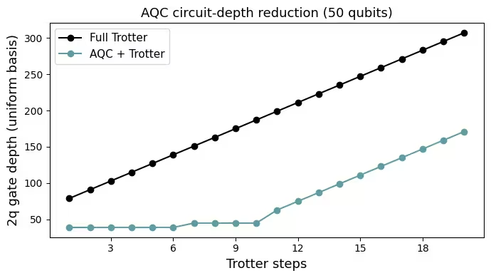
สำหรับฮาร์ดแวร์จริง วงจร Trotter ข้างต้นจะลึกเกินไป Approximate quantum compiling (AQC) แก้ปัญหานี้โดยการแทนที่ชั้น Trotter แรก $k$ ชั้น (รวมถึงวงจร ground state) ด้วย ansatz ที่มีพารามิเตอร์ที่สั้นกว่าซึ่งถูก optimize เพื่อ maximize fidelity ระดับ MPS กับวงจรลึกต้นฉบับ Trotter step ที่เหลือจะถูกต่อเข้าไปอย่างแน่นอน ทำให้ได้วงจร "AQC + Trotter" ที่ตื้นกว่า

เพื่อสร้างสมดุลระหว่าง expressibility กับความลึกของวงจร มีการใช้ ansatz สองแบบ: ansatz ชั้นเดียว (สร้างจาก Trotter step เดียว) บีบอัด time step แรกสุด และ ansatz สองชั้น ที่ลึกกว่า (สร้างจาก Trotter step สอง step) บีบอัด step ถัดไปไม่กี่ step ที่ต้องการ fidelity สูงกว่า

Workflow ของ AQC มีสี่ sub-step:

1. สร้างวงจรเป้าหมาย — วงจรแรก $k_1 + k_2$ วงจรจาก Step 1 ทำหน้าที่เป็นเป้าหมาย AQC โดยตรง

2. คำนวณ MPS เป้าหมาย — จำลองวงจรเป้าหมายแต่ละวงจรเป็น matrix-product state โดยใช้ quimb.tensor.CircuitMPS

3. สร้างและ optimize ansätze — generate_ansatz_from_circuit สร้าง ansatz แบบมีพารามิเตอร์หนึ่งชั้นและสองชั้น; พารามิเตอร์ถูก optimize โดยใช้ L-BFGS-B พร้อม gradient ที่เร่งด้วย JAX เพื่อ minimize $1 - |\langle\psi_{\mathrm{ansatz}}|\psi_{\mathrm{target}}\rangle|^2$ step แรก $k_1$ step ใช้ ansatz ชั้นเดียวและ step ถัดไป $k_2$ step ใช้ ansatz สองชั้น; ภายในแต่ละ stage แต่ละ step จะ warm-start จากพารามิเตอร์ที่ optimize แล้วของ step ก่อนหน้า และพารามิเตอร์จะถูกรีเซ็ตเป็นค่า default ของ stage ที่ขอบเขตของ stage

4. ประกอบวงจรแบบผสม — สำหรับ time step ที่เกิน checkpoint ของ AQC ให้ต่อชั้น Trotter แบบ exact (ไม่ประมาณ) เข้ากับวงจร AQC สองชั้นที่ optimize แล้วโดยใช้ trotter_evolution

# Number of time steps to compress into an AQC ansatz with one layer
aqc_n_steps_1 = 3
# Number of time steps to compress into an AQC ansatz with two layers
aqc_n_steps_2 = 2
aqc_n_steps_total = aqc_n_steps_1 + aqc_n_steps_2

# ── Step 2a: Target circuits (first aqc_n_steps_total circuits from Step 1) ──
target_circuits = {
    k: circuits[k - 1] for k in range(1, aqc_n_steps_total + 1)
}
# ── Step 2b: Compute target MPS ──
# Decompose PauliEvolutionGate to RXX/RYY/RZZ before passing to the AQC MPS
# backend, which does not understand PauliEvolutionGate natively.
aqc_sim = QuimbSimulator(
    quimb_circuit_factory=partial(
        qtn.CircuitMPS,
        gate_opts=dict(max_bond=mps_max_bond, cutoff=mps_cutoff),
    ),
    autodiff_backend="jax",
)
print("\nStep 2b — target MPS:")
target_mps = {}
for k in range(1, aqc_n_steps_total + 1):
    target_mps[k] = tensornetwork_from_circuit(
        target_circuits[k].decompose(["PauliEvolution"]), aqc_sim
    )
    print(f"  k={k}: max bond = {target_mps[k].psi.max_bond()}")

# ── Step 2c: Generate ansätze (one-layer and two-layer) and optimize parameters ──
ansatz_1, initial_params_1 = generate_ansatz_from_circuit(
    target_circuits[1].decompose(["PauliEvolution"]),
    qubits_initially_zero=True,
)
initial_params_1 = np.array(initial_params_1)
ansatz_2, initial_params_2 = generate_ansatz_from_circuit(
    target_circuits[2].decompose(["PauliEvolution"]),
    qubits_initially_zero=True,
)
initial_params_2 = np.array(initial_params_2)
print(
    f"\nStep 2c — one-layer ansatz: {ansatz_1.num_parameters} parameters, "
    f"2q depth (uniform basis) = {uniform_2q_depth(ansatz_1)}"
)
print(
    f"Step 2c — two-layer ansatz: {ansatz_2.num_parameters} parameters, "
    f"2q depth (uniform basis) = {uniform_2q_depth(ansatz_2)}"
)

aqc_circuits = {}
aqc_params = {}
for k in range(1, aqc_n_steps_total + 1):
    if k <= aqc_n_steps_1:
        ansatz, base_params = ansatz_1, initial_params_1
    else:
        ansatz, base_params = ansatz_2, initial_params_2
    # Warm-start from the previous step only within the same stage
    same_stage = (k - 1 >= 1) and (
        (k - 1 <= aqc_n_steps_1) == (k <= aqc_n_steps_1)
    )
    x0 = aqc_params[k - 1] if same_stage else base_params
    obj = MaximizeStateFidelity(target_mps[k], ansatz, aqc_sim)
    t0 = timeit.default_timer()
    result = scipy.optimize.minimize(
        obj.loss_function,
        x0,
        method="L-BFGS-B",
        jac=True,
        options=dict(maxiter=100),
    )
    elapsed = timeit.default_timer() - t0
    aqc_params[k] = result.x
    aqc_circuits[k] = ansatz.assign_parameters(result.x)
    print(
        f"  k={k}: fidelity = {1 - result.fun:.4f}, "
        f"2q depth (uniform basis) = "
        f"{uniform_2q_depth(aqc_circuits[k])}, "
        f"{elapsed:.1f}s"
    )

# ── Step 2d: Assemble full circuit set (AQC + Trotter) ──
all_circuits = []
for k in range(1, aqc_n_steps_total + 1):
    all_circuits.append(aqc_circuits[k])
base = aqc_circuits[aqc_n_steps_total]
for k in range(1, n_steps - aqc_n_steps_total + 1):
    circuit = base.copy()
    for instr in trotter_evolution(
        circuit.qubits, interaction, anisotropy, time_step, k
    ):
        circuit.append(instr)
    all_circuits.append(circuit)

full_depths = [
    uniform_2q_depth(circuits[k - 1]) for k in range(1, n_steps + 1)
]
aqc_depths = [uniform_2q_depth(circuit) for circuit in all_circuits]
full_2q = [
    circuits[k - 1].decompose(["PauliEvolution"]).num_nonlocal_gates()
    for k in range(1, n_steps + 1)
]
aqc_2q = [
    circuit.decompose(["PauliEvolution"]).num_nonlocal_gates()
    for circuit in all_circuits
]
print(f"\nStep 2d — assembled {len(all_circuits)} circuits")
print(
    f"  At step {n_steps} (uniform basis): "
    f"Trotter 2q depth = {full_depths[-1]}, AQC+Trotter 2q depth = {aqc_depths[-1]}; "
    f"2q gates: Trotter = {full_2q[-1]}, AQC+Trotter = {aqc_2q[-1]}"
)

steps_axis = np.arange(1, n_steps + 1)
fig, ax = plt.subplots(figsize=(7, 4))
ax.plot(steps_axis, full_depths, "-o", color="black", label="Full Trotter")
ax.plot(
    steps_axis, aqc_depths, "-o", color="cadetblue", label="AQC + Trotter"
)
ax.set_xlabel("Trotter steps", fontsize=13)
ax.xaxis.set_major_locator(plt.matplotlib.ticker.MaxNLocator(integer=True))
ax.set_ylabel("2q gate depth (uniform basis)", fontsize=13)
ax.set_title(f"AQC circuit-depth reduction ({n_qubits} qubits)", fontsize=13)
ax.legend(fontsize=11)
plt.tight_layout()
plt.show()

Step 2b — target MPS:
  k=1: max bond = 22
  k=2: max bond = 22
  k=3: max bond = 26
  k=4: max bond = 27
  k=5: max bond = 30

Step 2c — one-layer ansatz: 389 parameters, 2q depth (uniform basis) = 27
Step 2c — two-layer ansatz: 470 parameters, 2q depth (uniform basis) = 33
  k=1: fidelity = 1.0000, 2q depth (uniform basis) = 27, 11.8s
  k=2: fidelity = 0.9980, 2q depth (uniform basis) = 27, 13.2s
  k=3: fidelity = 0.9890, 2q depth (uniform basis) = 27, 13.7s
  k=4: fidelity = 0.9983, 2q depth (uniform basis) = 33, 16.4s
  k=5: fidelity = 0.9957, 2q depth (uniform basis) = 33, 16.4s

Step 2d — assembled 10 circuits
  At step 10 (uniform basis): Trotter 2q depth = 163, AQC+Trotter 2q depth = 99; 2q gates: Trotter = 371, AQC+Trotter = 200

Step 3: Execute โดยใช้ Qiskit primitives

เราจำลองวงจรที่ AQC-compile แล้วแต่ละวงจรโดยใช้ primitive StatevectorEstimator

estimator = StatevectorEstimator()
pubs = [(circuit, observables) for circuit in all_circuits]
job = estimator.run(pubs)
result = job.result()

Step 4: ประมวลผลภายหลังและคืนผลลัพธ์ในรูปแบบคลาสสิกตามต้องการ

ตอนนี้เราดึงค่าคาดหวัง $\langle\sigma_i^z\rangle$ สำหรับทุก qubit $i$ ในแต่ละ time step $t$ ค่าเหล่านี้ประกอบเป็นเมทริกซ์ retarded Green's function $G^R(j, j_c, t)$ จากนั้นเราแปลงฟูริเยร์ RGF ให้เป็น dynamical structure factor $S(q, \omega)$ และพล็อตทั้ง RGF และ DSF get_dsf ใช้ mirror symmetry และตัดค่าลบทิ้งภายในตัวมันเอง

rgf_mat = np.stack([pub_result.data.evs for pub_result in result])

# -- Compute DSF --
n_points_momentum, n_points_frequency = 100, 100
spectrum = get_dsf(
    n_qubits,
    rgf_mat,
    time_step,
    n_steps,
    n_points_momentum,
    n_points_frequency,
)

# -- Plot retarded Green's function --
plot_rgf(
    n_qubits,
    rgf_mat,
    time_step,
    n_steps,
    title=f"Retarded Green's function — {n_qubits} qubits (simulation)",
)

# -- Plot DSF --
plot_dsf(
    spectrum,
    time_step,
    n_points_momentum,
    n_points_frequency,
    title=f"Dynamical structure factor — {n_qubits} qubits (simulation)",
)

การ execute บนฮาร์ดแวร์ขนาดใหญ่

ตอนนี้เราขยายขนาดขึ้นเป็น 50 qubit ที่ scale นี้ การ optimize จะได้ fidelity ต่ำกว่าตัวอย่างขนาดเล็ก: fidelity ของ ansatz ground state ลดลงเหลือประมาณ 0.65 และ fidelity ของ AQC ลดลงเหลือประมาณ 0.7 ที่ checkpoint ในช่วงหลัง นี่เป็นสิ่งที่คาดไว้ และคุณสามารถปรับปรุง fidelity เหล่านี้ได้โดยการเพิ่มจำนวนชั้น ansatz ของ ground state (gs_n_layers) หรือจำนวน iteration ของการ optimize (maxiter) โดยแลกกับต้นทุนการคำนวณแบบคลาสสิกเพิ่มเติม โปรดสังเกตด้วยว่า fidelity ของ AQC สองชั้นออกมาต่ำกว่าแบบชั้นเดียว นี่ไม่ใช่การถดถอย: time step ในช่วงหลังสร้าง entanglement มากขึ้นและบีบอัดได้ยากกว่า จึงเป็นเหตุผลที่ใช้ ansatz สองชั้นที่มี expressibility มากกว่าสำหรับ step เหล่านั้น

การ optimize AQC อาจใช้เวลาคำนวณแบบคลาสสิกหลายชั่วโมง (ประมาณหกชั่วโมงในรันที่แสดงที่นี่ ส่วนใหญ่ใช้ไปกับ checkpoint สองชั้นใน Step 2c) เพื่อลดเวลา wall-clock ให้พิจารณารัน notebook นี้บนฮาร์ดแวร์แบบคลาสสิกที่ทรงพลังกว่า เช่นระบบ high-performance computing (HPC) หรืออีกทางหนึ่ง คุณสามารถลดขนาดปัญหาให้เล็กลงได้ (เช่น qubit น้อยลงหรือ time step น้อยลง); ผลลัพธ์ของคุณจะแตกต่างจากที่แสดงที่นี่

โค้ดด้านล่างเป็นไปตามโครงสร้างสี่ step เดียวกันกับตัวอย่างขนาดเล็ก พารามิเตอร์ ground state ของ HVA ถูก optimize อีกครั้งโดยใช้การจำลองด้วย MPS บน QPU เราเปิดใช้งาน dynamical decoupling (DD), Pauli twirling และ twirled readout error extinction (TREX) สำหรับการระงับและลดข้อผิดพลาด ตารางต่อไปนี้สรุปว่าการทดลองขนาดใหญ่แตกต่างจากขนาดเล็กอย่างไร:

	ขนาดเล็ก	ขนาดใหญ่
Qubit	10	50
Time step	10	20
AQC checkpoint (1-layer + 2-layer)	3 + 2 = 5	6 + 4 = 10
ชั้น ansatz ของ ground state	3	5
MPS max bond dimension	32	128
Estimator	StatevectorEstimator	QPU พร้อม DD, Pauli twirling และ TREX

ข้อความ XLA compile ช้า

ระหว่างการ optimize AQC (Step 2c ด้านล่าง) คุณอาจเห็นข้อความ stderr เช่น:

[Compiling module jit_MakeArrayFn for CPU] Very slow compile? ...
The operation took 2m14s

สิ่งเหล่านี้เป็น diagnostic ที่ไม่เป็นอันตรายจาก XLA ซึ่งเป็น compiler ที่รองรับ JAX autodiff ของ qiskit-addon-aqc-tensor ที่ 50 qubit ด้วย MPS bond dimension 128 XLA ใช้เวลาสองสามนาทีในการ compile ฟังก์ชัน gradient ในครั้งแรกที่ถูก trace การ compile สำเร็จ และผลลัพธ์ของการ optimize ไม่ได้รับผลกระทบ

# ── Parameters ──────────────────────────────────────────────────────────────
n_qubits = 50  # 10 → 50
interaction = 1.0  # J
anisotropy = 1.0  # ε (isotropic point)
time_step = 0.6
n_steps = 20  # 10 → 20
aqc_n_steps_1 = 6  # 3 → 6
aqc_n_steps_2 = 4  # 2 → 4
aqc_n_steps_total = aqc_n_steps_1 + aqc_n_steps_2
gs_n_layers = 5  # 3 → 5
mps_max_bond = 128  # 32 -> 128
mps_cutoff = 1e-8
center = n_qubits // 2 - 1

# ── Step 1: Map ──────────────────────────────────────────────────────────────
ham_mpo = xxz_hamiltonian_mpo(n_qubits, interaction, anisotropy)

dmrg = qtn.DMRG2(ham_mpo)
dmrg.solve(tol=1e-8)
print(f"Ground-state energy (DMRG): {dmrg.energy:.6f}")

gs_ansatz = build_ground_state_ansatz(n_qubits, gs_n_layers)

rng = np.random.default_rng(12345)
x0 = np.tile([0.0, np.pi / 2], gs_n_layers) + rng.normal(
    scale=0.1, size=2 * gs_n_layers
)
print("Optimizing ground state ansatz...")
t0 = timeit.default_timer()
result = optimize_ground_state_ansatz(
    gs_ansatz,
    x0,
    dmrg.state,
    max_bond=mps_max_bond,
    cutoff=mps_cutoff,
    options=dict(maxiter=100),
)
t1 = timeit.default_timer()
print(f"Finished optimizing ground state ansatz in {t1 - t0} seconds.")
print(f"Ground state ansatz fidelity: {1 - result.fun:.6f}")

gs_circuit = gs_ansatz.assign_parameters(result.x)
gs_circuit_mps = quimb_circuit(
    gs_circuit.decompose(["PauliEvolution"]),
    quimb_circuit_class=qtn.CircuitMPS,
    max_bond=mps_max_bond,
    cutoff=mps_cutoff,
)
gs_ansatz_energy = qtn.expec_TN_1D(
    gs_circuit_mps.psi.H, ham_mpo, gs_circuit_mps.psi
)
print(f"Ground state ansatz energy: {gs_ansatz_energy:.6f}")

perturbed = gs_circuit.copy()
perturbed.rz(np.pi / 2, center)

circuits = []
for t in range(1, n_steps + 1):
    circuit = perturbed.copy()
    for instr in trotter_evolution(
        circuit.qubits, interaction, anisotropy, time_step, t
    ):
        circuit.append(instr)
    circuits.append(circuit)
print(
    f"Built {len(circuits)} circuits, deepest 2q depth (uniform basis) = "
    f"{uniform_2q_depth(circuits[-1])}"
)

observables = [
    SparsePauliOp.from_sparse_list([("Z", [i], 1)], num_qubits=n_qubits)
    for i in range(n_qubits)
]
print(f"Defined {len(observables)} Z observables.")

# ── Step 2: AQC ──────────────────────────────────────────────────────────────
target_circuits = {
    k: circuits[k - 1] for k in range(1, aqc_n_steps_total + 1)
}

aqc_sim = QuimbSimulator(
    quimb_circuit_factory=partial(
        qtn.CircuitMPS,
        gate_opts=dict(max_bond=mps_max_bond, cutoff=mps_cutoff),
    ),
    autodiff_backend="jax",
)
print("\nStep 2b — target MPS:")
target_mps = {}
for k in range(1, aqc_n_steps_total + 1):
    target_mps[k] = tensornetwork_from_circuit(
        target_circuits[k].decompose(["PauliEvolution"]), aqc_sim
    )
    print(f"  k={k}: max bond = {target_mps[k].psi.max_bond()}")

ansatz_1, initial_params_1 = generate_ansatz_from_circuit(
    target_circuits[1].decompose(["PauliEvolution"]),
    qubits_initially_zero=True,
)
initial_params_1 = np.array(initial_params_1)
ansatz_2, initial_params_2 = generate_ansatz_from_circuit(
    target_circuits[2].decompose(["PauliEvolution"]),
    qubits_initially_zero=True,
)
initial_params_2 = np.array(initial_params_2)
print(
    f"\nStep 2c — one-layer ansatz: {ansatz_1.num_parameters} parameters, "
    f"2q depth (uniform basis) = {uniform_2q_depth(ansatz_1)}"
)
print(
    f"Step 2c — two-layer ansatz: {ansatz_2.num_parameters} parameters, "
    f"2q depth (uniform basis) = {uniform_2q_depth(ansatz_2)}"
)

aqc_circuits = {}
aqc_params = {}
for k in range(1, aqc_n_steps_total + 1):
    if k <= aqc_n_steps_1:
        ansatz, base_params = ansatz_1, initial_params_1
    else:
        ansatz, base_params = ansatz_2, initial_params_2
    # Warm-start from the previous step only within the same stage
    same_stage = (k - 1 >= 1) and (
        (k - 1 <= aqc_n_steps_1) == (k <= aqc_n_steps_1)
    )
    x0 = aqc_params[k - 1] if same_stage else base_params
    obj = MaximizeStateFidelity(target_mps[k], ansatz, aqc_sim)
    t0 = timeit.default_timer()
    result = scipy.optimize.minimize(
        obj.loss_function,
        x0,
        method="L-BFGS-B",
        jac=True,
        options=dict(maxiter=100),
    )
    elapsed = timeit.default_timer() - t0
    aqc_params[k] = result.x
    aqc_circuits[k] = ansatz.assign_parameters(result.x)
    print(
        f"  k={k}: fidelity = {1 - result.fun:.4f}, "
        f"2q depth (uniform basis) = "
        f"{uniform_2q_depth(aqc_circuits[k])}, "
        f"{elapsed:.1f}s"
    )

all_circuits = []
for k in range(1, aqc_n_steps_total + 1):
    all_circuits.append(aqc_circuits[k])
base = aqc_circuits[aqc_n_steps_total]
for k in range(1, n_steps - aqc_n_steps_total + 1):
    circuit = base.copy()
    for instr in trotter_evolution(
        circuit.qubits, interaction, anisotropy, time_step, k
    ):
        circuit.append(instr)
    all_circuits.append(circuit)

full_depths = [
    uniform_2q_depth(circuits[k - 1]) for k in range(1, n_steps + 1)
]
aqc_depths = [uniform_2q_depth(circuit) for circuit in all_circuits]
full_2q = [
    circuits[k - 1].decompose(["PauliEvolution"]).num_nonlocal_gates()
    for k in range(1, n_steps + 1)
]
aqc_2q = [
    circuit.decompose(["PauliEvolution"]).num_nonlocal_gates()
    for circuit in all_circuits
]
print(f"\nStep 2d — assembled {len(all_circuits)} circuits")
print(
    f"  At step {n_steps} (uniform basis): "
    f"Trotter 2q depth = {full_depths[-1]}, AQC+Trotter 2q depth = {aqc_depths[-1]}; "
    f"2q gates: Trotter = {full_2q[-1]}, AQC+Trotter = {aqc_2q[-1]}"
)

steps_axis = np.arange(1, n_steps + 1)
fig, ax = plt.subplots(figsize=(7, 4))
ax.plot(steps_axis, full_depths, "-o", color="black", label="Full Trotter")
ax.plot(
    steps_axis, aqc_depths, "-o", color="cadetblue", label="AQC + Trotter"
)
ax.set_xlabel("Trotter steps", fontsize=13)
ax.xaxis.set_major_locator(plt.matplotlib.ticker.MaxNLocator(integer=True))
ax.set_ylabel("2q gate depth (uniform basis)", fontsize=13)
ax.set_title(f"AQC circuit-depth reduction ({n_qubits} qubits)", fontsize=13)
ax.legend(fontsize=11)
plt.tight_layout()
plt.show()

# ── Step 3: Execute on IBM Quantum hardware ───────────────────────────────────
# (replaces StatevectorEstimator)
service = QiskitRuntimeService()
backend = service.least_busy(
    min_num_qubits=n_qubits,
    operational=True,
    simulator=False,
    filters=lambda x: x.configuration().processor_type["family"] == "Heron",
)
print(f"Backend: {backend.name}")

pm = generate_preset_pass_manager(optimization_level=3, backend=backend)
isa_circuits = pm.run(all_circuits, num_processes=1)
isa_2q_depths = [
    isa_circuit.depth(lambda inst: inst.operation.num_qubits == 2)
    for isa_circuit in isa_circuits
]
print(
    f"Transpiled 2q depth (deepest, ISA on {backend.name}): "
    f"{max(isa_2q_depths)} "
    f"(2q gates: {max(isa_circuit.num_nonlocal_gates() for isa_circuit in isa_circuits)})"
)

estimator = Estimator(backend)
estimator.options.environment.job_tags = ["TUT_SNS"]
estimator.options.dynamical_decoupling.enable = True
estimator.options.dynamical_decoupling.sequence_type = "XY4"
estimator.options.twirling.enable_gates = True
estimator.options.twirling.num_randomizations = 1000
estimator.options.twirling.shots_per_randomization = 128
estimator.options.resilience.measure_mitigation = True
estimator.options.resilience.measure_noise_learning.num_randomizations = 32
estimator.options.resilience.measure_noise_learning.shots_per_randomization = 100

pubs = [
    (
        isa_circuit,
        [obs.apply_layout(isa_circuit.layout) for obs in observables],
    )
    for isa_circuit in isa_circuits
]
job = estimator.run(pubs)
print(f"Job ID: {job.job_id()}")

result = job.result()

# ── Step 4: Post-process ──────────────────────────────────────────────────────
rgf_mat = np.stack([pub_result.data.evs for pub_result in result])

n_points_momentum, n_points_frequency = 100, 100
spectrum = get_dsf(
    n_qubits,
    rgf_mat,
    time_step,
    n_steps,
    n_points_momentum,
    n_points_frequency,
)

plot_rgf(
    n_qubits,
    rgf_mat,
    time_step,
    n_steps,
    title=f"Retarded Green's function — {n_qubits} qubits (QPU)",
)
plot_dsf(
    spectrum,
    time_step,
    n_points_momentum,
    n_points_frequency,
    title=rf"KCuF$_3$ DSF — {n_qubits} qubits (QPU)"
    "\n(AQC + DD + Pauli twirling + TREX)",
)

Ground-state energy (DMRG): -21.972109
Optimizing ground state ansatz...
Finished optimizing ground state ansatz in 132.2076231740648 seconds.
Ground state ansatz fidelity: 0.645956
Ground state ansatz energy: -21.616744
Built 20 circuits, deepest 2q depth (uniform basis) = 307
Defined 50 Z observables.

Step 2b — target MPS:
  k=1: max bond = 44
  k=2: max bond = 46
  k=3: max bond = 53
  k=4: max bond = 62
  k=5: max bond = 75
  k=6: max bond = 96
  k=7: max bond = 118
  k=8: max bond = 128
  k=9: max bond = 128
  k=10: max bond = 128

Step 2c — one-layer ansatz: 2971 parameters, 2q depth (uniform basis) = 39
Step 2c — two-layer ansatz: 3412 parameters, 2q depth (uniform basis) = 45
  k=1: fidelity = 1.0000, 2q depth (uniform basis) = 39, 215.6s
  k=2: fidelity = 0.9676, 2q depth (uniform basis) = 39, 269.8s
  k=3: fidelity = 0.9014, 2q depth (uniform basis) = 39, 293.5s
  k=4: fidelity = 0.8755, 2q depth (uniform basis) = 39, 279.6s
  k=5: fidelity = 0.8450, 2q depth (uniform basis) = 39, 266.4s
  k=6: fidelity = 0.8146, 2q depth (uniform basis) = 39, 371.0s

E0626 02:59:07.229070 1508496 slow_operation_alarm.cc:73] 
********************************
[Compiling module jit_MakeArrayFn for CPU] Very slow compile? If you want to file a bug, run with envvar XLA_FLAGS=--xla_dump_to=/tmp/foo and attach the results.
********************************
E0626 02:59:21.713796 1508477 slow_operation_alarm.cc:140] The operation took 2m14.484932074s

********************************
[Compiling module jit_MakeArrayFn for CPU] Very slow compile? If you want to file a bug, run with envvar XLA_FLAGS=--xla_dump_to=/tmp/foo and attach the results.
********************************

k=7: fidelity = 0.7312, 2q depth (uniform basis) = 45, 10865.3s
  k=8: fidelity = 0.7720, 2q depth (uniform basis) = 45, 1450.3s
  k=9: fidelity = 0.7316, 2q depth (uniform basis) = 45, 3388.6s

E0626 07:21:05.148724 1508496 slow_operation_alarm.cc:73] 
********************************
[Compiling module jit_MakeArrayFn for CPU] Very slow compile? If you want to file a bug, run with envvar XLA_FLAGS=--xla_dump_to=/tmp/foo and attach the results.
********************************
E0626 07:21:24.286095 1508477 slow_operation_alarm.cc:140] The operation took 2m19.137566498s

********************************
[Compiling module jit_MakeArrayFn for CPU] Very slow compile? If you want to file a bug, run with envvar XLA_FLAGS=--xla_dump_to=/tmp/foo and attach the results.
********************************

k=10: fidelity = 0.6726, 2q depth (uniform basis) = 45, 3396.1s

Step 2d — assembled 20 circuits
  At step 20 (uniform basis): Trotter 2q depth = 307, AQC+Trotter 2q depth = 171; 2q gates: Trotter = 3775, AQC+Trotter = 1913

Backend: ibm_fez
Transpiled 2q depth (deepest, ISA on ibm_fez): 105 (2q gates: 2574)
Job ID: d8v39vhropqc738biotg

ผลลัพธ์จากฮาร์ดแวร์สร้างลักษณะสำคัญของ two-spinon continuum ขึ้นมาใหม่: ความเข้มการกระเจิงกระจุกตัวอยู่ใกล้ antiferromagnetic wave vector $q = \pi$ ที่พลังงานต่ำ และถูกจำกัดจากด้านล่างด้วย spinon dispersion แบบไซน์ พร้อมด้วย continuum ของ spectral weight ที่กว้างอยู่เหนือมันแทนที่จะเป็น mode เดียวที่คมชัด นี่เป็นโครงสร้างเดียวกับที่วัดได้ด้วย inelastic neutron scattering บน KCuF$_3$ และมันตรวจสอบความถูกต้องของ workflow เต็มรูปแบบของการเตรียม ground state, perturbation, Trotter evolution ที่บีบอัดด้วย AQC และการวัดที่ผ่านการลดข้อผิดพลาด (error mitigation) ที่ scale 50-qubit

ขั้นตอนถัดไป

หากคุณพบว่างานนี้น่าสนใจ คุณอาจสนใจเนื้อหาต่อไปนี้:

คำแนะนำ

• จำลองการกระเจิงนิวตรอนด้วย AQC + Trotter dynamics Serverless workflow — tutorial คู่กันที่รันการทดลองเดียวกันนี้ผ่านฟังก์ชัน template ของ Qiskit Serverless ที่ deploy แล้ว

• Lee et al., "Benchmarking quantum simulation with neutron-scattering experiments" (arXiv:2603.15608) — งานวิจัยอ้างอิงที่ tutorial นี้อ้างอิงจาก

• เทคนิคการลด (mitigation) และระงับ (suppression) ข้อผิดพลาด — DD, Pauli twirling และ TREX ที่ใช้ในการทดลองฮาร์ดแวร์

• Approximate quantum compilation สำหรับวงจร time evolution — tutorial เกี่ยวกับ AQC-Tensor

• เอกสาร AQC-Tensor