Shadow tomography ของสถานะ Greenberger-Horne-Zeilinger

ประมาณการการใช้งาน: ไม่ถึง 10 วินาทีบนโปรเซสเซอร์ Heron r2 (หมายเหตุ: นี่เป็นเพียงค่าประมาณ เวลารันจริงของคุณอาจแตกต่างไป)

ผลลัพธ์การเรียนรู้

• shadow tomography สร้าง classical shadow ของสถานะควอนตัมได้อย่างไร และทำไมจึงต้องใช้การวัดน้อยกว่า full state tomography แบบเอกซ์โพเนนเชียล

• วิธีทำ local Pauli shadow tomography โดยใช้ Qiskit เพื่อประมาณค่าแมกเนไทเซชันของคิวบิตเดี่ยว, correlator สองจุด และ reduced density matrix ของสองคิวบิต

• วิธีใช้ qiskit-paulice สำหรับการตรวจจับ error แบบ overhead ต่ำโดยใช้ spacetime code ในการทดลองฮาร์ดแวร์ขนาดใหญ่

ความรู้พื้นฐานที่ต้องมี

• การวัด

• Quantum state tomography

• การตรวจจับ error โดยใช้ spacetime code

ความเป็นมา

Full quantum state tomography ของระบบ $N$ คิวบิตต้องใช้การวัดจำนวนมากแบบเอกซ์โพเนนเชียลเพื่อประมาณพารามิเตอร์อิสระทั้งหมด $4^N -1$ ตัวของ density matrix ตัวอย่างเช่น สำหรับระบบ 50 คิวบิต กระบวนการนี้ต้องใช้ shot ในระดับ $10^{30}$ ซึ่งมากกว่าจำนวนดาวฤกษ์ในเอกภพที่สังเกตได้มากกว่าพันล้านเท่า Shadow tomography [1] เป็นโปรโตคอลสารสนเทศควอนตัมที่สร้าง “classical shadow” ของสถานะควอนตัม ซึ่งใช้ประมาณค่า observable เป้าหมายได้ด้วยจำนวน shot ที่เพิ่มขึ้นเป็นลอการิทึมตามจำนวน observable และไม่ขึ้นกับขนาดระบบ $N$ ทำให้เกี่ยวข้องกับหลายสาขาในการคำนวณควอนตัม เช่น การประมาณพลังงาน เอนโทรปีของ entanglement และการคำนวณฟังก์ชันสหสัมพันธ์ การประมาณ kernel ใน quantum machine learning และอื่นๆ

บทเรียนนี้แสดงวิธีใช้ shadow tomography เพื่อประมาณ observable เฉพาะที่ เช่น แมกเนไทเซชันของคิวบิตเดี่ยว $\langle Z_i \rangle$ สำหรับคิวบิต $i$, ฟังก์ชันสหสัมพันธ์สองจุด $\langle Z_i Z_j\rangle$ และ reduced density matrix ของสองคิวบิต (2-RDM) ของสถานะ Greenberger-Horne-Zeilinger (GHZ) ที่พัวพันกันสูง บทเรียนเริ่มด้วยการแสดง workflow ของ shadow tomography ขนาดเล็กบนสถานะ GHZ 10 คิวบิตโดยใช้การจำลอง statevector จากนั้นแสดงการสาธิต 100 คิวบิตบนฮาร์ดแวร์ควอนตัมจริง

โปรโตคอล shadow tomography

โปรโตคอล shadow tomography มีขั้นตอนดังนี้:

1. ใช้ unitary แบบสุ่ม $U$ ที่สุ่มจาก unitary ensemble กับสถานะควอนตัมเริ่มต้น
2. วัดผลใน computational basis จะได้ bitstring $\ket{b}$
3. เก็บ classical snapshot $\hat{\rho} = \mathcal{M}^{-1}(U^{\dagger}\ket{b}\bra{b}U)$ โดยที่ $\mathcal{M}^{-1}$ คือตัวผกผันของ measurement channel $\mathcal{M}(\rho)=\mathbb{E}[U^{\dagger}\ket{b}\bra{b}U]$
4. ทำซ้ำกระบวนการ $T$ ครั้ง โดยที่ชุดของ snapshot $T$ ตัว $\{\hat{\rho}_t\}$ ก่อให้เกิด classical shadow $S(\rho, T)$
5. ประมาณค่า observable $o$ ของตัวดำเนินการ $O$ เป็น $\frac{1}{T}\sum_{t=1}^{T}\text{Tr}(O\hat{\rho}_t)$

รูปแบบต่างๆ ของ shadow tomography

การเลือก unitary ensemble หรือก็คือ basis ในขั้นตอนที่ 1 ของโปรโตคอล ส่งผลต่อ sample complexity ความแปรปรวนของค่าประมาณ และความสมบูรณ์ของข้อมูลของ shadow tomography นั้นๆ มีการพิจารณากลุ่ม ensemble มากมายในงานวิจัย แต่ละแบบมีข้อแลกเปลี่ยนระหว่างความซับซ้อนและประสิทธิภาพในการประมาณ observable คุณสมบัติของรูปแบบที่ใช้บ่อยที่สุดสรุปไว้ในตารางต่อไปนี้ แม้รายการนี้จะไม่ครบถ้วน

รูปแบบ	Ensemble	Sample complexity	ความลึกของ circuit	Observable ที่เหมาะสม
local Pauli [1]	Pauli คิวบิตเดี่ยว $\{X, Y, Z\}$	$\mathcal{O}(3^k\text{log}M/\varepsilon^2)$	1	เฉพาะที่/few-body
global Clifford [1]	Clifford $N$ คิวบิต	$\mathcal{O}(\text{Tr}(O^2)\text{log}M/\varepsilon^2)$	$\mathcal{O}(N\text{log}N)$	low-rank, fidelity
fermionic Gaussian [2], [3]	matchgate circuit	$\mathcal{O}(\binom{\mu}{k}\frac{1}{\varepsilon^2})$	$\mathcal{O}(N^2)$	fermionic
shallow shadows [4], [5]	circuit ความลึกต่ำ	$\mathcal{O}(k2^k\text{log}M/\varepsilon^2)$	$\mathcal{O}(\text{log}N)$	ไม่เฉพาะที่ (เหมาะกับฮาร์ดแวร์)

คำศัพท์ที่ใช้ในตารางมีความหมายดังนี้:

• "sample complexity" หมายถึงจำนวนการวัดที่ต้องใช้สำหรับ shadow tomography รูปแบบนั้นๆ

• "ความลึกของ circuit" อธิบายว่าการวัดมีค่าใช้จ่ายสูงเพียงใดในการทำบนฮาร์ดแวร์ควอนตัม

• $N$ คือจำนวนคิวบิต

• $k$ คือความเป็นเฉพาะที่ (locality) ของ observable (เช่น $\langle Z_i \rangle$ มี $k=1$ และ $\langle Z_i Z_j\rangle$ มี $k=2$)

• $M$ คือจำนวน observable ที่ต้องการประมาณพร้อมกัน

• $\varepsilon$ คือค่าความคลาดเคลื่อนแบบบวกที่ยอมรับได้

• $\mu$ คือจำนวนเฟอร์มิออน

แม้ local Pauli ensemble จะเหมาะกับฮาร์ดแวร์ที่สุด แต่ก็ต้องจ่ายค่าปรับ sample complexity เป็น $3^k$ ทำให้ไม่เหมาะกับการประมาณคุณสมบัติที่ไม่เฉพาะที่ โดยทั่วไปแล้ว ขอบเขต sample complexity ของ local shadow เพิ่มตาม $4^k$ และดีขึ้นเป็น $3^k$ ในกรณีพิเศษของ observable แบบ tensor-product

ในทางกลับกัน แม้ global Clifford ensemble จะใช้ประมาณ observable ที่ไม่เฉพาะที่ได้ แต่ความลึกของ circuit ไม่เอื้ออำนวย Fermionic Gaussian shadow มีประโยชน์ในการจำลองฟิสิกส์หลายวัตถุ เคมี และวัสดุ แต่ต้องใช้ matchgate circuit ซึ่งอาจมี overhead สูงบนอุปกรณ์แบบ gate ทั่วไป

Shallow shadows มีความลึกของ circuit อยู่ระหว่าง local Pauli และ global Clifford ทำให้เป็นรูปแบบที่น่าสนใจมากสำหรับการใช้งานจริง แม้ยังมีคำถามเปิดบางข้อเกี่ยวกับความลึกของ circuit ที่เหมาะสมที่สุดสำหรับ observable หนึ่งๆ

ขณะที่แนวหน้าของงานวิจัย shadow tomography ขยายตัวต่อไป ปัญหาที่เกี่ยวข้องที่สุดบางข้อที่ต้องแก้ ได้แก่ การเลือก measurement ensemble ที่เหมาะสมที่สุดสำหรับชุด observable เป้าหมาย การปรับปรุงขอบเขต sample complexity และการขยายโปรโตคอลไปยัง observable ที่วิวัฒน์ตามเวลา อย่างไรก็ตาม shadow tomography ยังคงเป็นหนึ่งใน workflow ชั้นนำสำหรับดึงข้อมูลคลาสสิกสูงสุดจากสถานะควอนตัมโดยใช้การวัดน้อยที่สุด ซึ่งทำให้เหมาะอย่างยิ่งสำหรับการระบุลักษณะของสถานะควอนตัมในสเกลที่ทั้ง full tomography และการจำลองแบบคลาสสิกเป็นไปไม่ได้

Local Pauli ensemble

บทเรียนนี้ใช้ basis แบบ Pauli สุ่ม หรือก็คือ Clifford gate คิวบิตเดี่ยว เพื่อเก็บ shadow และประมาณคุณสมบัติของสถานะ GHZ โปรดทราบว่าการวัดแบบ Pauli เป็นตัวเลือกที่ยอดเยี่ยมสำหรับการประมาณ observable เฉพาะที่ (เช่น ความหนาแน่นสปิน ฟังก์ชันสหสัมพันธ์เฉพาะที่ และความหนาแน่นความน่าจะเป็นของตำแหน่ง) แต่ไม่เหมาะกับ observable ระดับโลก (เช่น พลังงานรวม โมเมนตัม และประจุ)

ที่นี่ จะสุ่มเลือก basis แบบ Pauli $\{X, Y, Z\}$ ต่อคิวบิตอย่างเป็นอิสระต่อกัน แล้วใช้การหมุนคิวบิตเดี่ยวที่สอดคล้องกัน ตามด้วยการวัด:

$$\begin{equation} U = U_0 \otimes U_1 \otimes \cdots \otimes U_{n-1}, U_q \in \{I, H, S^{\dagger}H\} \end{equation} \tag{1}$$

สำหรับ ensemble นี้ ตัวผกผันของ measurement channel คือ:

$$\begin{equation} \hat{\rho}_q=3U_q^{\dagger}\ket{b_q}\bra{b_q}U_q - I \end{equation} \tag{2}$$

ตัวคูณ $3$ มาจากการเฉลี่ยบน basis แบบ Pauli ทั้งสาม ซึ่งให้ depolarizing channel ที่มีพารามิเตอร์ $\frac{1}{3}$ จากนั้น estimator เต็มรูปจะแยกตัวประกอบเป็นผลคูณของ estimator คิวบิตเดี่ยว ดังที่แสดงในตาราง สำหรับ observable $M$ ตัว แต่ละตัวมี locality $k$ จำนวน Pauli shadow ที่ต้องใช้เพื่อประมาณ observable ทั้งหมดให้ได้ความคลาดเคลื่อนแบบบวก $\varepsilon$ ด้วยความน่าจะเป็นสูงคือ $\mathcal{O}(\frac{3^k\text{log}(M)}{\varepsilon^2})$ ขนาดของระบบไม่มีผลต่อต้นทุนการวัด ตราบใดที่ observable ยังเป็นเฉพาะที่ ดังนั้นจึงประมาณ observable จำนวนมากแบบเอกซ์โพเนนเชียลพร้อมกันได้ด้วยต้นทุนเพียงระดับลอการิทึม

Median of means

ค่าเฉลี่ยธรรมดาบน snapshot $T$ ตัวลดความแปรปรวนของค่าประมาณ observable จากการวัดครั้งเดียวเป็น $\frac{1}{T}$ แต่ไวต่อค่านอกเกณฑ์ (outlier) สามารถใช้ median of means เพื่อแก้ปัญหานี้ได้ กระบวนการประกอบด้วย:

• แบ่ง snapshot $T$ ตัวออกเป็น $K$ กลุ่มขนาดเท่ากัน
• คำนวณค่าเฉลี่ยภายในแต่ละกลุ่ม
• คืนค่ามัธยฐานของค่าเฉลี่ยของกลุ่มทั้งหมด

บทเรียนนี้ทำ local Pauli shadow tomography เพื่อประมาณคุณสมบัติของสถานะ GHZ โดยเริ่มจากตัวอย่างจำลอง 10 คิวบิต แล้วสาธิตการทดลองบนฮาร์ดแวร์ 100 คิวบิต

ข้อกำหนด

ก่อนเริ่มบทเรียนนี้ ตรวจสอบให้แน่ใจว่าคุณติดตั้งสิ่งต่อไปนี้แล้ว:

• Qiskit SDK v2.0 ขึ้นไป พร้อมรองรับ visualization

• IBM Quantum Compute v0.28 ขึ้นไป (pip install qiskit-ibm-runtime)

• Qiskit Paulice (pip install qiskit-paulice)

การตั้งค่า

# Added by doQumentation — installs the packages this notebook needs if they are missing
import importlib.util

_needed = {"matplotlib": "matplotlib", "numpy": "numpy", "qiskit": "qiskit", "qiskit_ibm_runtime": "qiskit-ibm-runtime", "qiskit_paulice": "qiskit-paulice"}
_missing = [pip for module, pip in _needed.items()
            if importlib.util.find_spec(module) is None]
# One at a time, so a package that fails to install does not block the others
for _pip in _missing:
    %pip install -q {_pip}
if not _missing:
    print("\u2713 All required packages are installed")

import numpy as np
import matplotlib.pyplot as plt
from collections import deque, defaultdict
from qiskit import QuantumCircuit, ClassicalRegister
from qiskit.quantum_info import (
    Statevector,
    partial_trace,
    Operator,
    Pauli,
    SparsePauliOp,
)
from qiskit.transpiler import generate_preset_pass_manager
from qiskit_ibm_runtime import QiskitRuntimeService
from qiskit_ibm_runtime import SamplerV2 as Sampler
from qiskit_paulice.layout import get_low_overhead_ancillas

seed = 42  # for reproducibility
rng = np.random.default_rng(seed)

ฟังก์ชันช่วยเหลือต่อไปนี้ถูกใช้ในตัวอย่างฮาร์ดแวร์ขนาดใหญ่ในตอนหลังของบทเรียน:

• bad_cz, bad_readout, bad_coherence — สอบถามข้อมูลการสอบเทียบของ backend เพื่อระบุ gate, คิวบิต และ edge ที่เกินเกณฑ์ error หรือ coherence เพื่อให้ตัดออกจาก layout ของ circuit ได้

• parallel_ghz — สร้าง circuit GHZ ตามขนาดที่กำหนดโดยใช้ breadth-first search บน coupling map โดยกระจายเลเยอร์ CNOT แบบขนานเพื่อลดความลึกของ circuit

• weighted_coverage, active_wires, z_trace_backward — คำนวณว่าพื้นผิว error ของ circuit GHZ ได้รับการป้องกันมากเพียงใดโดยชุดการตรวจสอบพาริตีแบบ spacetime ที่กำหนด โดยใช้เทคนิค backward-propagation จาก [6]

• add_measurements — เพิ่มการวัดของคิวบิต GHZ และคิวบิตตรวจสอบลงใน classical register แยกกัน เพื่อให้ postselect ได้อย่างเป็นอิสระ

• build_shadow_circuits — สร้างหนึ่ง circuit ต่อหนึ่ง basis แบบ Pauli สุ่ม โดยเพิ่มการหมุนคิวบิตเดี่ยวที่เหมาะสมก่อนการวัด

• parse_hw_results_w_checks — แกะเอาต์พุตของ Sampler เป็นชุดสามค่า (ghz_bits, check_bits, bases) หนึ่งชุดต่อหนึ่ง shot

• adapt_to_flat_bits, estimate_zz_nn_hw — แมปบิตของ register GHZ กลับไปยังพื้นที่ดัชนีของอุปกรณ์ทั้งหมด และคำนวณค่าประมาณ median-of-means ของ $\langle Z_i Z_{i+1}\rangle$

def bad_cz(target, threshold: float = 0.01) -> list:
    "Return edges whose CZ error exceeds threshold."
    edges = []
    for edge in backend.target.build_coupling_map().get_edges():
        if (edge[1], edge[0]) not in edges:
            edges.append(edge)
    cz_errors = {edge: target["cz"][edge].error for edge in edges}
    worst = sorted(cz_errors.items(), key=lambda x: x[1], reverse=True)
    return [list(edge) for edge, error in worst if error > threshold]

def bad_readout(target, threshold: float = 0.01) -> list:
    "Return nodes whose measurement error exceeds threshold."
    meas_errors = {
        node: target["measure"][(node,)].error
        for node in range(backend.num_qubits)
    }
    worst = sorted(meas_errors.items(), key=lambda x: x[1], reverse=True)
    return [node for node, error in worst if error > threshold]

def bad_coherence(target, threshold: float = 60) -> list:
    "Return nodes whose T2 value is below threshold."
    t2s = {
        node: (target.qubit_properties[node].t2 or 0) * 1e6
        for node in range(backend.num_qubits)
    }
    return [
        node
        for node, val in sorted(t2s.items(), key=lambda x: x[1])
        if val < threshold
    ]

def parallel_ghz(
    root: int, num_qubits: int, backend, bad_edges: list, skip: list
) -> tuple:
    "Build a GHZ circuit of size num_qubits using BFS from root, one neighbor per layer."
    edges = [
        e
        for e in [list(e) for e in backend.coupling_map.get_edges()]
        if e not in bad_edges
        and [e[1], e[0]] not in bad_edges
        and e[0] not in skip
        and e[1] not in skip
    ]
    adj = defaultdict(list)
    for u, v in edges:
        adj[u].append(v)
        adj[v].append(u)

    qc = QuantumCircuit(backend.num_qubits)
    visited = [root]
    queue = deque([root])
    explored = defaultdict(set)
    layers = []
    qc.h(root)

    while queue and len(visited) < num_qubits:
        layer = []
        for node in list(queue):
            queue.popleft()
            unvisited = [
                nb
                for nb in adj[node]
                if nb not in visited and nb not in explored[node]
            ]
            if unvisited:
                nb = unvisited[0]
                visited.append(nb)
                queue.append(node)
                queue.append(nb)
                explored[node].add(nb)
                layer.append((node, nb))
                if len(visited) == num_qubits:
                    break
        if layer:
            layers.append(layer)
        else:
            break

    for layer in layers:
        for q1, q2 in layer:
            qc.cx(q1, q2)
        qc.barrier()

    return qc, visited, layers

def weighted_coverage(
    layers: list, parities: list, w_idle: float = 0.2, w_gate: float = 0.8
) -> float:
    "Compute weighted fraction of wires covered by at least one parity check."
    wires = active_wires(layers)
    covered_by_any = {n_layer: set() for n_layer in range(len(layers))}
    for parity in parities:
        for n_layer, qs in z_trace_backward(layers, parity).items():
            covered_by_any[n_layer] |= qs
    covered_weight = total_weight = 0
    for n_layer in range(len(layers)):
        idle = wires[n_layer]["idle"]
        gate = wires[n_layer]["gate"]
        total_weight += w_idle * len(idle) + w_gate * len(gate)
        covered_weight += w_idle * len(
            covered_by_any[n_layer] & idle
        ) + w_gate * len(covered_by_any[n_layer] & gate)
    return covered_weight / total_weight if total_weight > 0 else 0

def active_wires(layers: list) -> dict:
    """
    Returns per-layer dict with two sets:
    - 'idle': activated wires that are idle in this layer
    - 'gate': activated wires that are control/target of a CNOT at this layer
    """
    first_activation = {}
    for n_layer, layer in enumerate(layers):
        for c, t in layer:
            first_activation.setdefault(c, n_layer)
            first_activation.setdefault(t, n_layer)
    result = {}
    for n_layer in range(len(layers)):
        active = {
            q
            for q, n_layer0 in first_activation.items()
            if n_layer >= n_layer0
        }
        gate = {q for c, t in layers[n_layer] for q in (c, t)}
        result[n_layer] = {"idle": active - gate, "gate": gate}
    return result

def z_trace_backward(layers: list, initial_Zs: list) -> dict:
    """
    Backward propagate Zs with parity cancellation.
    Returns {layer: set of qubits with odd parity Z at that layer}.
    """
    wires = active_wires(layers)
    support = set(initial_Zs)
    trace = {}
    for n_layer in range(len(layers) - 1, -1, -1):
        active = wires[n_layer]["idle"] | wires[n_layer]["gate"]
        trace[n_layer] = support & active
        new_support = set()
        for q in support:
            hit = False
            for c, t in layers[n_layer]:
                if q == t:
                    new_support ^= {t, c}
                    hit = True
                    break
                elif q == c:
                    new_support ^= {c}
                    hit = True
                    break
            if not hit:
                new_support ^= {q}
        support = new_support
    return trace

def add_measurements(
    qc: QuantumCircuit, ghz_qubits: list, checks: list
) -> QuantumCircuit:
    "Add GHZ and check qubit measurements into separate classical registers."
    c1 = ClassicalRegister(len(ghz_qubits), "c1")
    qc.add_register(c1)
    for q, c in zip(ghz_qubits, c1):
        qc.measure(q, c)
    c2 = ClassicalRegister(len(checks), "c2")
    qc.add_register(c2)
    for q, c in zip(checks, c2):
        qc.measure(q, c)
    return qc

def build_shadow_circuits(
    base_circuit: QuantumCircuit,
    n_measure: int,
    ghz_qubits: list,
    checks: list,
) -> tuple:
    "Build n_measure circuits by appending random Pauli basis rotations to each GHZ qubit."
    n = base_circuit.num_qubits
    all_bases = rng.integers(0, 3, size=(n_measure, n))
    circuits = []
    for m in range(n_measure):
        qc = base_circuit.copy()
        qc.barrier()
        for q in ghz_qubits:
            b = all_bases[m, q]
            if b == 1:
                qc.h(q)
            elif b == 2:
                qc.sdg(q)
                qc.h(q)
        add_measurements(qc, ghz_qubits, checks)
        circuits.append(qc)
    return circuits, all_bases

def parse_hw_results_w_checks(
    result, bases: np.ndarray, ghz_qubits: list, checks: list
) -> list:
    "Parse hardware bitstrings into (ghz_bits, check_bits, bases) triples."
    snapshots = []
    n_ghz = len(ghz_qubits)
    n_checks = len(checks)
    for t, pub_result in enumerate(result):
        ghz_strings = (
            pub_result.data.c1.get_bitstrings()
        )  # one entry per shot
        chk_strings = pub_result.data.c2.get_bitstrings()
        for ghz_bitstring, check_bitstring in zip(ghz_strings, chk_strings):
            ghz_bits = [
                int(ghz_bitstring[n_ghz - 1 - i]) for i in range(n_ghz)
            ]
            check_bits = [
                int(check_bitstring[n_checks - 1 - i])
                for i in range(n_checks)
            ]
            snapshots.append((ghz_bits, check_bits, bases[t]))
    return snapshots

def adapt_to_flat_bits(
    ghz_bits: list, ghz_qubits: list, n_total: int
) -> list:
    "Map GHZ-register bits back to a full n_total-length bit vector."
    bits = [0] * n_total
    for i, q in enumerate(ghz_qubits):
        bits[q] = ghz_bits[i]
    return bits

def estimate_zz_nn_hw(
    snapshots: list, ghz_qubits: list, n_total: int, n_groups: int
) -> np.ndarray:
    "Estimate <ZiZi+1> for each neighboring GHZ qubit pair from flat-bit snapshots."
    pairs = list(zip(ghz_qubits[:-1], ghz_qubits[1:]))
    all_est = np.column_stack(
        [
            snapshot_estimate(
                ["Z" if q in pair else "I" for q in range(n_total)], snapshots
            )
            for pair in pairs
        ]
    )
    return mom(all_est, n_groups).real

ตัวอย่างตัวจำลองขนาดเล็ก

ก่อนอื่น เตรียมสถานะ GHZ 10 คิวบิตโดยใช้การจำลอง statevector และประมาณคุณสมบัติของมันโดยใช้ local Pauli shadow สถานะ GHZ เป็นสถานะควอนตัมที่พัวพันสูงสุดตั้งแต่สามคิวบิตขึ้นไป ใช้เป็น benchmark สำหรับ entanglement หลายส่วน และเป็นองค์ประกอบพื้นฐานที่พบบ่อยของโปรโตคอลการสื่อสารและการเข้ารหัสลับเชิงควอนตัม นอกจากนี้ circuit GHZ ยังมีคุณสมบัติเชิงวิเคราะห์ที่ทราบครบถ้วน จึงเหมาะอย่างยิ่งสำหรับการตรวจสอบในบทเรียนนี้

ขั้นตอนที่ 1: แมปอินพุตแบบคลาสสิกเป็นปัญหาควอนตัม

เตรียมสถานะ GHZ 10 คิวบิตในอุดมคติ

def ghz_statevector(num_qubits):
    qc = QuantumCircuit(num_qubits)
    qc.h(0)
    for q in range(num_qubits - 1):
        qc.cx(q, q + 1)
    return Statevector(qc)

num_qubits = 10  # number of qubits
psi = ghz_statevector(num_qubits)
psi.seed(seed)
print(
    f"{num_qubits}-qubit GHZ state ready (norm = {np.linalg.norm(psi):.6f})"
)

10-qubit GHZ state ready (norm = 1.000000)

ขั้นตอนที่ 2: ปรับให้เหมาะสมสำหรับการรันบนฮาร์ดแวร์ควอนตัม

ถัดไป กำหนดฟังก์ชันที่เก็บ shadow snapshot โดยหมุนสถานะ GHZ ไปยัง basis แบบ Pauli สุ่ม ซึ่งเลียนแบบสิ่งที่ Sampler primitive ทำบนฮาร์ดแวร์ในตัวอย่างขนาดใหญ่

def basis_circuit(b):
    """0 -> Z basis (I), 1 -> X basis (H), 2 -> Y basis (Sdg;H)."""
    qc = QuantumCircuit(1)
    if b == 1:
        qc.h(0)
    elif b == 2:
        qc.sdg(0)
        qc.h(0)
    # b == 0: Z basis, no rotation
    return qc

_basis = {
    b: basis_circuit(b) for b in (0, 1, 2)
}  # built once, shared with the estimator's _U

def collect_shadow_snapshots(psi, n_snapshots, num_qubits):
    snapshots = []
    for _ in range(n_snapshots):
        bases = rng.integers(0, 3, size=num_qubits)
        rot = QuantumCircuit(num_qubits)
        for q, b in enumerate(bases):
            rot.compose(_basis[b], qubits=[q], inplace=True)
        evolved = psi.evolve(rot)
        evolved.seed(int(rng.integers(0, 2**31)))
        bitstr = next(
            iter(evolved.sample_counts(shots=1))
        )  # Born rule internal
        bits = [int(x) for x in bitstr[::-1]]  # little-endian -> qubit
        snapshots.append((bits, bases))
    return snapshots

ขั้นตอนที่ 3: รันโดยใช้ Qiskit primitive

สำหรับการจำลองนี้ ใช้ statevector โดยตรง

n_snapshots = 5000  # number of shadow snapshots
n_groups = 20  # groups/batches for median-of-means

snapshots = collect_shadow_snapshots(psi, n_snapshots, num_qubits)
print(f"Collected {n_snapshots} snapshots.")

Collected 5000 snapshots.

ขั้นตอนที่ 4: ประมวลผลภายหลังและคืนผลลัพธ์ในรูปแบบคลาสสิกที่ต้องการ

กำหนด shadow estimator และ median-of-means (MOM) estimator สำหรับฐานการวัดแบบสุ่มที่ใช้เก็บ shadow snapshot ใช้ฟังก์ชันเหล่านี้เพื่อประมาณคุณสมบัติของสถานะ GHZ จากผลการวัดที่เก็บมา ซึ่งรวมถึงแมกเนไทเซชันของ Qubit เดี่ยว ตัวสัมพันธ์สอง Qubit และ RDM สอง Qubit จากนั้นเปรียบเทียบค่าที่ประมาณได้กับค่าที่แน่นอน

_U = {
    b: Operator(basis_circuit(b)) for b in (0, 1, 2)
}  # rotation Uᵢ per basis
_P = {p: Operator(Pauli(p)) for p in "IXYZ"}  # single-qubit Paulis

def shadow_estimator(P, b, bit):  # P is a label char, e.g. "X"
    UPU = _U[b] @ _P[P] @ _U[b].adjoint()  # Uᵢ P Uᵢ†
    return (3 * UPU.data[bit, bit] - np.trace(_P[P].data)).real

def mom(estimates: np.ndarray, n_groups: int) -> np.ndarray:
    "Median-of-means outlier suppression."
    T = len(estimates)
    spg = T // n_groups  # shots per group
    trimmed = estimates[
        : spg * n_groups
    ]  # drop any leftover shots that don't cleanly fit into a group
    groups = trimmed.reshape(n_groups, spg, *estimates.shape[1:])
    means = groups.mean(axis=1)  # take the mean of each group
    return np.median(means.real, axis=0) + 1j * np.median(
        means.imag, axis=0
    )  # take the median of means for real and imaginary parts separately

def snapshot_estimate(
    pauli_string, snapshots
):  # full-width label, len == num_qubits
    out = np.empty(len(snapshots), dtype=complex)
    for t, (bits, bases) in enumerate(snapshots):
        e = 1.0 + 0j
        for q, P in enumerate(pauli_string):
            e *= shadow_estimator(P, bases[q], bits[q])
        out[t] = e
    return out

Z_est = np.column_stack(
    [
        snapshot_estimate(
            ["Z" if q == i else "I" for q in range(num_qubits)], snapshots
        )
        for i in range(num_qubits)
    ]
)
Z_vals = mom(Z_est, n_groups).real

ZZ_est = np.column_stack(
    [
        snapshot_estimate(
            ["Z" if q in (i, i + 1) else "I" for q in range(num_qubits)],
            snapshots,
        )
        for i in range(num_qubits - 1)
    ]
)
ZZ_nn = mom(ZZ_est, n_groups).real

ZZ_full = np.zeros((n_snapshots, num_qubits, num_qubits), dtype=complex)
for i in range(num_qubits):
    ZZ_full[:, i, i] = 1.0  # diagonal is always 1
    for j in range(i + 1, num_qubits):
        col = snapshot_estimate(
            ["Z" if q in (i, j) else "I" for q in range(num_qubits)],
            snapshots,
        )
        ZZ_full[:, i, j] = col
        ZZ_full[:, j, i] = col  # symmetric
ZZ_mat = mom(ZZ_full, n_groups).real

# 2-qubit reduced density matrix (RDM) for pair (qi, qj)
# the elementwise complex median (real/imag split) for the RDM coefficients generalizes the scalar median in Ref.[1]
qi, qj = 0, num_qubits - 1
terms = []
for a in "IXYZ":
    for b in "IXYZ":
        label = "".join({qi: a, qj: b}.get(q, "I") for q in range(num_qubits))
        c = mom(snapshot_estimate(label, snapshots).reshape(-1, 1), n_groups)[
            0
        ]
        terms.append((b + a, c / 4))
rho_shadow = SparsePauliOp.from_list(terms).to_matrix()

traced_out = [q for q in range(num_qubits) if q not in (qi, qj)]
rho_exact = partial_trace(
    psi, traced_out
).data  # diag(0.5, 0, 0, 0.5) for GHZ

print(f"{'Observable':<22} {'Estimated':>12} {'Ideal':>8} {'Max error':>12}")
print("-" * 57)
print(
    f"{'<Zi> (all qubits)':<22} {'-':>12} {'0':>8} {np.max(np.abs(Z_vals)):>12.4f}"
)
print(
    f"{'<ZiZi+1> mean':<22} {np.mean(ZZ_nn):>12.4f} {'1':>8} {np.max(np.abs(ZZ_nn - 1)):>12.4f}"
)
print(
    f"{'2-RDM Frobenius err':<22} {'-':>12} {'0':>8} {np.linalg.norm(rho_shadow - rho_exact):>12.4f}"
)

Observable                Estimated    Ideal    Max error
---------------------------------------------------------
<Zi> (all qubits)                 -        0       0.0540
<ZiZi+1> mean                1.0040        1       0.1520
2-RDM Frobenius err               -        0       0.1080

แสดงผลลัพธ์เป็นภาพ

กราฟแรกแสดงค่าแมกเนไทเซชันของ Qubit เดี่ยวที่ประมาณได้สำหรับแต่ละ Qubit กราฟที่สองแสดงการกระจายของค่าตัวสัมพันธ์สองจุดที่ประมาณได้สำหรับทุกคู่ Qubit กราฟสุดท้ายแสดงขนาดของสมาชิกในเมทริกซ์ความหนาแน่นลดรูปสอง Qubit เนื่องจากใช้ snapshot จำนวนค่อนข้างมากเมื่อเทียบกับขนาดระบบ ผลลัพธ์จึงใกล้เคียงกับค่าที่แน่นอนมาก

fig, axes = plt.subplots(
    1, 3, figsize=(14, 4), gridspec_kw={"width_ratios": [1, 1, 1]}
)

z_exact = psi.expectation_value(
    SparsePauliOp.from_sparse_list([("Z", [0], 1.0)], num_qubits)
).real  # 0.0
zz_exact = psi.expectation_value(
    SparsePauliOp.from_sparse_list([("ZZ", [0, 1], 1.0)], num_qubits)
).real  # 1.0

# <Zi>
axes[0].bar(range(num_qubits), Z_vals, color="#4a90d9", alpha=0.85)
axes[0].axhline(0, color="black", lw=0.8)
axes[0].set_ylim(-0.5, 0.5)
axes[0].set_title(r"$\langle Z_i \rangle$ (ideal = %0.2f)" % z_exact)
axes[0].set_xlabel("Qubit index")
axes[0].grid(axis="y", alpha=0.3)

# <ZiZj>
im = axes[1].imshow(ZZ_mat, vmin=-1, vmax=1, cmap="magma")
plt.colorbar(im, ax=axes[1])
axes[1].set_title(r"$\langle Z_i Z_j \rangle$ (ideal = %0.2f)" % zz_exact)
axes[1].set_xlabel("Qubit j")
axes[1].set_ylabel("Qubit i")

# 2-RDM magnitude
im2 = axes[2].imshow(np.abs(rho_shadow), vmin=0, vmax=0.5, cmap="Blues")
plt.colorbar(im2, ax=axes[2])
axes[2].set_title(r"$|\rho_2|$ for qubits (0, N-1)")
axes[2].set_xticks(range(4))
axes[2].set_yticks(range(4))
axes[2].set_xticklabels(["00", "01", "10", "11"])
axes[2].set_yticklabels(["00", "01", "10", "11"])

[Text(0, 0, '00'), Text(0, 1, '01'), Text(0, 2, '10'), Text(0, 3, '11')]

ประเมินการสเกลตามจำนวน shot

ในบทเรียนนี้ใช้ snapshot 5,000 ตัวเพื่อประมาณ observable เราประเมินการสเกลตามจำนวน shot ของ shadow tomography โดยพล็อตค่าความคลาดเคลื่อนเฉลี่ยของฟังก์ชันที่ประมาณได้ตัวหนึ่งเทียบกับงบจำนวน shot ที่ต่างกัน ความคลาดเคลื่อนของตัวสัมพันธ์สอง Qubit ลดลงตาม $1/\sqrt{T}$ ซึ่งเป็นไปตามที่คาดไว้สำหรับการลู่เข้าทางสถิติมาตรฐานของ mean estimator ความสำคัญของ shadow tomography คือสัมประสิทธิ์คงที่ที่คูณหน้า $1/\sqrt{T}$ ไม่เพิ่มขึ้นตามจำนวน Qubit สำหรับ observable เชิงท้องถิ่น เช่นที่ตรวจสอบในบทเรียนนี้

shot_counts = [100, 250, 500, 1000, 2000, 5000, 10000]
errors = []

for N_test in shot_counts:
    snaps = collect_shadow_snapshots(psi, N_test, num_qubits)
    zz_vals = []
    for i in range(num_qubits - 1):
        ests = []
        for bits, bases in snaps:
            e = 1.0 + 0j
            for q in range(num_qubits):
                op = "Z" if q in (i, i + 1) else "I"
                e *= shadow_estimator(op, bases[q], bits[q])
            ests.append(e.real)
        zz_vals.append(np.mean(ests))
    errors.append(float(np.mean(np.abs(np.array(zz_vals) - 1.0))))
    print(f"T={N_test:5d} error = {errors[-1]:.4f}")

fig, ax = plt.subplots(figsize=(6, 4))
T_arr = np.array(shot_counts, dtype=float)
ax.loglog(T_arr, errors, "o-", color="#4a90d9", lw=2, label="Shadow estimate")
ax.loglog(
    T_arr,
    errors[0] * np.sqrt(shot_counts[0] / T_arr),
    "k--",
    alpha=0.5,
    label=r"$1/\sqrt{T}$ reference",
)
ax.set_xlabel("Shots T")
ax.set_ylabel(r"Mean $|\langle Z_i Z_{i+1} \rangle - 1|$")
ax.set_title(f"Convergence for {num_qubits}-qubit GHZ")
ax.legend()
plt.tight_layout()
plt.show()

T=  100 error = 0.1856
T=  250 error = 0.1613
T=  500 error = 0.1027
T= 1000 error = 0.0827
T= 2000 error = 0.0513
T= 5000 error = 0.0311
T=10000 error = 0.0162

ตัวอย่างบนฮาร์ดแวร์ขนาดใหญ่

การจำลองก่อนหน้านี้ยืนยันว่า local Pauli shadow tomography กู้คืน observable ที่ถูกต้องได้บน statevector ที่ไม่มีสัญญาณรบกวน การรันโปรโตคอลเดียวกันด้วย 100 Qubit บนฮาร์ดแวร์จริงทำให้เกิดความท้าทายสองข้อที่ไม่ปรากฏในการจำลอง คือ ข้อผิดพลาดของ Gate และการอ่านค่าสะสมไปตามวงจร GHZ ที่ลึก และการหา layout ของ Qubit ที่เหมาะสมที่สุดต้องค้นหาในกราฟการเชื่อมต่อของอุปกรณ์ แทนที่จะเลือก layout ด้วยมือ

เพื่อรับมือกับความท้าทายข้อแรก ให้ใช้การตรวจจับข้อผิดพลาดแบบ low-overhead ด้วย spacetime codes [6] โดยใช้ ancilla Qubit จำนวนเล็กน้อยที่อยู่ติดกับต้นไม้ GHZ เป็น parity check ancilla แต่ละตัวถูกพันกับเพื่อนบ้าน GHZ สองตัวก่อนการวัด ดังนั้นข้อผิดพลาดแบบ bit-flip เพียงครั้งเดียวที่เพื่อนบ้านตัวใดตัวหนึ่งจะพลิกผลลัพธ์ของ ancilla จาก 0 เป็น 1 snapshot ที่ check ancilla ตัวใดอ่านได้ 1 จะถูกทิ้ง เหลือชุดย่อยที่สะอาดกว่าสำหรับใช้ประมาณ $\langle Z_i Z_{i+1}\rangle$

ความท้าทายข้อที่สองจัดการโดยการค้นหา layout ของต้นไม้ GHZ ที่เป็นตัวเลือก แล้วเลือกอันที่ทำให้ parity-check coverage สูงสุด คือสัดส่วนของสายใน Circuit ที่ถูกตรวจสอบโดย check อย่างน้อยหนึ่งตัว ภายใต้การเพิ่มขึ้นของความลึกของ Circuit ที่ยอมรับได้

ขั้นตอนที่ 1-4 (ทำในโค้ดบล็อกเดียว)

ตอนนี้นำเวิร์กโฟลว์สี่ขั้นตอนเดียวกันไปใช้กับสถานะ GHZ 100 Qubit บนฮาร์ดแวร์ควอนตัมจริง โดยเพิ่มคุณสมบัติเฉพาะฮาร์ดแวร์สองอย่างที่ไม่เกิดขึ้นในการจำลอง

• ขั้นตอนที่ 1 ระบุลักษณะสัญญาณรบกวนของ Backend (ข้อผิดพลาดของ Gate ข้อผิดพลาดในการอ่านค่า และเวลา T2) เพื่อตัด Qubit และเอจที่ไม่น่าเชื่อถือออกจาก layout ของ Circuit

• ขั้นตอนที่ 2 ค้นหา layout ของต้นไม้ GHZ ที่เป็นไปได้ เพื่อหาอันที่ทำให้ parity-check coverage สูงสุดภายในความลึกของ Circuit ที่ยอมรับได้ แทนที่โซ่แบบง่ายที่ใช้ในการจำลอง

• ขั้นตอนที่ 3 สร้าง shadow circuit (หนึ่งวงจรต่อหนึ่งฐาน Pauli แบบสุ่ม) ทรานสไพล์เป็น Gate เนทีฟของฮาร์ดแวร์ และส่งไปยังพริมิทีฟ Sampler ด้วย shots=8 (แต่ละ Circuit สร้าง bitstring อิสระแปดตัว)

• ขั้นตอนที่ 4 เลือก snapshot ที่ check qubit ทั้งหมดอ่านได้ 0 (ตรวจไม่พบข้อผิดพลาด) ด้วย postselection จากนั้นประมาณ $\langle Z_i Z_{i+1}\rangle$ ทั้งแบบมีและไม่มี postselection เพื่อแสดงให้เห็นว่าการตรวจจับข้อผิดพลาดช่วยปรับปรุงผลได้

# ── Step 1: Map classical inputs to a quantum problem ─────────────────────────
service = QiskitRuntimeService()
backend = service.least_busy(
    operational=True, simulator=False, min_num_qubits=133
)
coupling_map = backend.target.build_coupling_map()
n_total = backend.num_qubits

thresh_cz, thresh_meas, thresh_t2 = 0.025, 0.15, 10
bad_edges = bad_cz(backend.target, threshold=thresh_cz)
bad_nodes_readout = bad_readout(backend.target, threshold=thresh_meas)
dead_qubits = bad_readout(backend.target, threshold=0.4)
bad_nodes = list(
    set(bad_nodes_readout)
    | set(bad_coherence(backend.target, threshold=thresh_t2))
)

# ── Step 2: Optimize for quantum hardware execution ───────────────────────────
# Search over starting qubits and random node-skip sets to find the GHZ layout
# with the best parity-check coverage within an acceptable circuit depth.
ghz_size = 100
max_skips, shuffles, max_depth_increase = 10, 200, 10
w_idle, w_gate = 0.2, 0.8

# Find the root that yields the shallowest GHZ — exclude bad_nodes from the start
best_root = None
base_depth = float("inf")
for root in range(backend.num_qubits):
    if root in bad_nodes:
        continue
    qc, ghz_qubits, _ = parallel_ghz(
        root, ghz_size, backend, bad_edges, bad_nodes
    )
    if len(ghz_qubits) != ghz_size:
        continue
    depth = qc.depth(lambda x: x.operation.num_qubits == 2)
    if depth < base_depth:
        best_root, base_depth = root, depth
if best_root is None:
    raise Exception(
        "No qualifying GHZ root layout found. Relax error thresholds."
    )

qc, ghz_qubits, layers = parallel_ghz(
    best_root, ghz_size, backend, bad_edges, bad_nodes
)

degree_two_nodes = [
    i
    for i in ghz_qubits
    if all(n in ghz_qubits for n in coupling_map.neighbors(i))
    and len(coupling_map.neighbors(i)) >= 2
]

best_covered_fraction = -1
best_qc = best_checks = best_parities = best_layers = best_ghz_qubits = None

for num_skips in range(max_skips):
    for _ in range(shuffles):
        skip_trial = list(
            rng.choice(degree_two_nodes, num_skips, replace=False)
        )
        qc, ghz_qubits, layers = parallel_ghz(
            best_root, ghz_size, backend, bad_edges, skip_trial + bad_nodes
        )
        if len(ghz_qubits) != ghz_size:
            continue
        depth = qc.depth(lambda x: x.operation.num_qubits == 2)
        checks, parities = [], []
        for ancilla, neighbors in get_low_overhead_ancillas(
            coupling_map, ghz_qubits
        ).items():
            if ancilla in dead_qubits:
                continue
            good_neighbors = [
                n
                for n in neighbors
                if [ancilla, n] not in bad_edges
                and [n, ancilla] not in bad_edges
            ]
            if len(good_neighbors) < 2:
                continue
            checks.append(ancilla)
            parities.append((good_neighbors[0], good_neighbors[1]))
            qc.cx(good_neighbors[0], ancilla)
            qc.cx(good_neighbors[1], ancilla)
        covered_fraction = weighted_coverage(
            layers=layers, parities=parities, w_idle=w_idle, w_gate=w_gate
        )
        if (
            covered_fraction > best_covered_fraction
            and depth <= base_depth + max_depth_increase
        ):
            best_covered_fraction = covered_fraction
            (
                best_qc,
                best_ghz_qubits,
                best_checks,
                best_parities,
                best_layers,
            ) = qc, ghz_qubits, checks, parities, layers

qc, ghz_qubits, checks, parities, layers = (
    best_qc,
    best_ghz_qubits,
    best_checks,
    best_parities,
    best_layers,
)
if len(ghz_qubits) != ghz_size:
    raise Exception("No GHZ found. Relax error thresholds.")

print(f"GHZ qubits: {ghz_qubits} ({len(ghz_qubits)})")
print(f"Check qubits: {checks} ({len(checks)})")
print(
    "Covered fraction (no idle): ",
    weighted_coverage(
        layers=layers, parities=parities, w_idle=0.0, w_gate=1.0
    ),
)

# ── Step 3: Execute using Qiskit primitives ───────────────────────────────────
# Build one shadow circuit per random Pauli basis, each repeated for shots_per_basis
# independent bitstrings. Transpile to hardware-native gates, then submit using the
# Sampler primitive. Each circuit yields shots_per_basis snapshots in that basis.
n_hw = 1000
shots_per_basis = 8  # multiple shots per basis circuit
shadow_circs, hw_bases = build_shadow_circuits(qc, n_hw, ghz_qubits, checks)
sampler = Sampler(backend)
sampler.options.environment.job_tags = ["TUT_STGHZS"]
pm = generate_preset_pass_manager(optimization_level=1, backend=backend)
isa_circuit = pm.run(shadow_circs)
job = sampler.run(isa_circuit, shots=shots_per_basis)
result = job.result()

# ── Step 4: Post-process and return result in desired classical format ─────────
# Filter snapshots whose check qubits all read 0 (no detected error), then
# estimate <ZiZi+1> with and without the error-detection postselection.
snapshots_hw = parse_hw_results_w_checks(result, hw_bases, ghz_qubits, checks)
snapshots_kept = [
    (ghz_bits, check_bits, bases)
    for (ghz_bits, check_bits, bases) in snapshots_hw
    if all(b == 0 for b in check_bits)
]
snapshots_kept_adapted = [
    (adapt_to_flat_bits(ghz_bits, ghz_qubits, n_total), bases)
    for (ghz_bits, check_bits, bases) in snapshots_kept
]
snapshots_hw_adapted = [
    (adapt_to_flat_bits(ghz_bits, ghz_qubits, n_total), bases)
    for (ghz_bits, check_bits, bases) in snapshots_hw
]

print("Shadow snapshots collected:", len(snapshots_hw))
print("Shadow snapshots kept post error-detection:", len(snapshots_kept))

n_groups = min(5, len(snapshots_kept))  # groups for median-of-means
ZZ_hw = estimate_zz_nn_hw(snapshots_hw_adapted, ghz_qubits, n_total, n_groups)
ZZ_kept = estimate_zz_nn_hw(
    snapshots_kept_adapted, ghz_qubits, n_total, n_groups
)

# Plot <ZiZi+1> before and after error detection
fig, axes = plt.subplots(1, 2, figsize=(13, 4))

axes[0].plot(ZZ_hw, "o-", color="#e05c5c", markersize=4)
axes[0].axhline(1.0, color="gray", ls="--", alpha=0.7, label="Ideal")
axes[0].set_ylim(-0.6, 3.0)
axes[0].set_title(r"$\langle Z_i Z_{i+1} \rangle$ (without error detection)")
axes[0].set_xlabel("GHZ qubit pair")
axes[0].legend()
axes[0].grid(alpha=0.3)

axes[1].plot(ZZ_kept, "o-", color="#e05c5c", markersize=4)
axes[1].axhline(1.0, color="gray", ls="--", alpha=0.7, label="Ideal")
axes[1].set_ylim(-0.6, 3.0)
axes[1].set_title(r"$\langle Z_i Z_{i+1} \rangle$ (with error detection)")
axes[1].set_xlabel("GHZ qubit pair")
axes[1].legend()
axes[1].grid(alpha=0.3)

plt.tight_layout()
plt.show()

print("Before detection: <ZiZi+1>= ", float(np.average(ZZ_hw)))
print("After detection: <ZiZi+1>= ", float(np.average(ZZ_kept)))

GHZ qubits: [57, 47, 67, 46, 66, 48, 45, 65, 49, 44, 64, 38, 43, 77, 29, 42, 85, 28, 56, 41, 84, 30, 27, 36, 86, 31, 21, 87, 32, 20, 88, 33, 22, 97, 89, 34, 23, 107, 78, 39, 35, 16, 106, 90, 69, 53, 19, 24, 3, 108, 105, 91, 70, 52, 15, 25, 2, 109, 104, 92, 71, 54, 51, 14, 4, 1, 110, 103, 98, 93, 58, 55, 13, 5, 0, 118, 96, 72, 59, 12, 6, 129, 102, 73, 11, 7, 128, 101, 74, 10, 8, 127, 100, 9, 126, 116, 125, 121, 124, 120] (100)
Check qubits: [68, 37, 50, 63, 83, 17, 26, 18, 117, 111, 75] (11)
Covered fraction (no idle):  0.5454545454545454
Shadow snapshots collected: 8000
Shadow snapshots kept post error-detection: 566

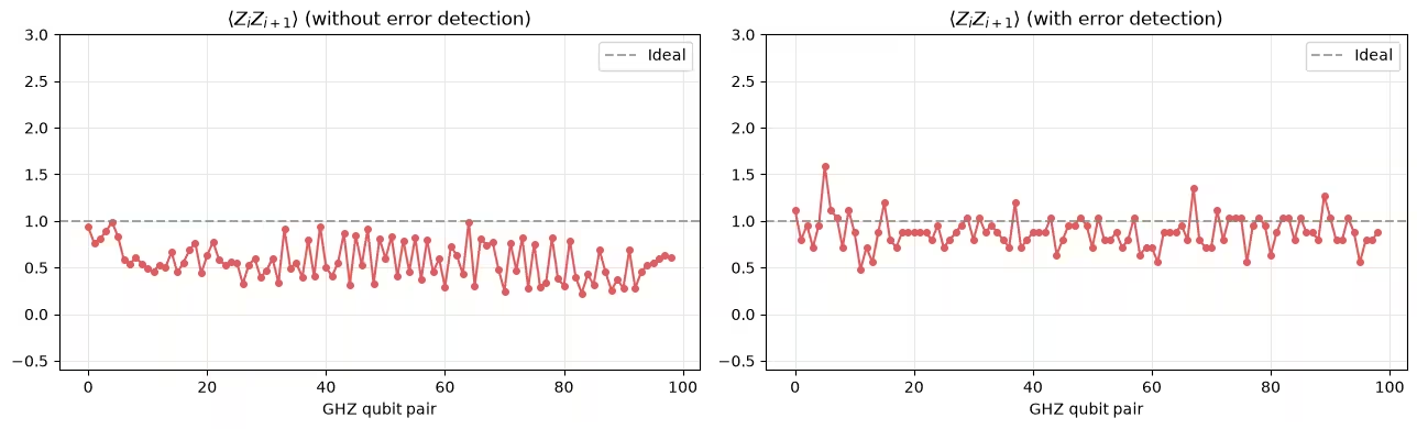
Before detection: <ZiZi+1>=  0.573749999999951
After detection: <ZiZi+1>=  0.8817377312951776

แปลผลลัพธ์

กราฟทั้งสองแสดง $\langle Z_i Z_{i+1}\rangle$ ที่ประมาณจาก shadow tomography สำหรับแต่ละคู่ Qubit ข้างเคียงในสาย GHZ 100 Qubit ก่อนและหลังการทำ postselection ตาม parity check

สำหรับสถานะ GHZ ในอุดมคติ ตัวสัมพันธ์ระหว่างเพื่อนบ้านใกล้สุดทั้งหมดเท่ากับ $1$ บนฮาร์ดแวร์ สัญญาณรบกวนทำให้ค่าประมาณดิบต่ำลงและเกิดการกระจายระหว่าง Qubit หลังการตรวจจับข้อผิดพลาด snapshot ที่เกิดข้อผิดพลาดที่ตรวจพบได้อย่างน้อยหนึ่งครั้งจะถูกตัดออก และค่าประมาณที่เหลือจะเข้าใกล้ $1$ มากขึ้นพร้อมความแปรปรวนที่ลดลง ซึ่งสอดคล้องกับสถานะที่มีประสิทธิภาพที่สะอาดกว่า

การปรับปรุงหลังการตรวจจับข้อผิดพลาดสอดคล้องกับการที่ check ตรวจพบข้อผิดพลาดจริง

ขั้นตอนต่อไป

สำรวจแหล่งข้อมูลต่อไปนี้เพื่อเรียนรู้เพิ่มเติม:

คำแนะนำ

• General formulation of quantum information
• Low-overhead error detection using spacetime codes tutorial
• Qiskit Paulice add-on API documentation

เอกสารอ้างอิง

• [1] Huang, H. Y., Kueng, R., & Preskill, J. (2020). Predicting many properties of a quantum system from very few measurements. Nature Physics, 16, 1050–1057.

• [2] Zhao, A., Rubin, N. C., & Miyake, A. (2021). Fermionic partial tomography via classical shadows. Phys. Rev. Lett., 127, 110504.

• [3] Low, G. H. (2022). Classical shadows of fermions with particle number symmetry. arXiv:2208.08964.

• [4] Bertoni, C., Haferkamp, J., Hinsche, M. et al. (2024). Shallow Shadows: Expectation Estimation Using Low-Depth Random Clifford Circuits. Phys. Rev. Lett., 133, 020602.

• [5] Hu, H.-Y., Gu, A., Majumder, S. et al. (2025). Demonstration of robust and efficient quantum property learning with shallow shadows. Nature Communications, 16, 2943.

• [6] Martiel, S. & Javadi-Abhari, A. (2025). Low-overhead error detection with spacetime codes. arXiv:2504.15725. © IBM Corp. 2026