การหา diagonalization เชิงควอนตัมแบบ pooled sample-based ของ Hamiltonian นิวเคลียส

ประมาณการใช้งาน: 2.5 นาทีบนโปรเซสเซอร์ Heron (หมายเหตุ: นี่เป็นเพียงการประมาณการ runtime ของคุณอาจแตกต่างออกไป)

กำลังมองหาเวอร์ชัน Fortran อยู่หรือ?

โน้ตบุ๊กนี้นำเสนอการ implement ด้วย Python การ implement ด้วย Fortran อยู่ใน ไดเรกทอรีคู่มือ Fortran ของ repository เอกสารนี้ เวอร์ชัน Python เพิ่มขั้นตอน self-consistent configuration-recovery ซึ่ง driver ของ Fortran ไม่ได้ทำ

ผลลัพธ์การเรียนรู้

• เรียนรู้ว่า nuclear shell-model Hamiltonian ที่จัดตารางในฐานของ orbital แบบ $J$-coupled กลายเป็น qubit Hamiltonian ใน $m$-scheme ได้อย่างไร โดยที่ qubit หนึ่งตัวคือ single-particle state หนึ่งสถานะ

• สร้าง excitation ansatz แบบคงที่ที่ไม่ใช่ variational ซึ่งมุมของมันมาจากทฤษฎี perturbation อันดับสอง ดังนั้นจึงไม่มี classical optimization loop

• เปรียบเทียบ excitation แบบ qubit และแบบ fermionic และวัดว่าการเลือกส่งผลต่อ two-qubit depth ของ ensemble อย่างไร

• รัน self-consistent configuration recovery ด้วย qiskit-addon-sqd เมื่อปริมาณที่อนุรักษ์ เป็นจำนวน nucleon, $M_J$ และ parity แทนที่จะเป็นจำนวนอิเล็กตรอนและสปิน

• นำ workflow หนึ่งไปใช้จากปัญหา 24 qubit ที่คุณสามารถตรวจสอบได้อย่างแม่นยำ ไปสู่ปัญหา 40 qubit ที่มี basis state เกือบสองล้านสถานะ ซึ่งเกินขีดความสามารถของ exact-diagonalization ในบทเรียนนี้

ข้อกำหนดเบื้องต้น

ก่อนเริ่มต้น โปรดทบทวนหัวข้อต่อไปนี้:

• การหา diagonalization เชิงควอนตัมแบบ sample-based และ เอกสารอ้างอิง API ของ addon SQD

• การหา diagonalization เชิงควอนตัมแบบ sample-based ของ Hamiltonian เคมี ซึ่งเป็นคู่เทียบเชิงโครงสร้างอิเล็กตรอนของบทเรียนนี้

• Transpile กับ backend target และ บทนำสู่ primitives

• Second quantization และการ mapping แบบ Jordan-Wigner

ความเป็นมา

nuclear shell model ถือว่านิวเคลียสประกอบด้วย nucleon valence จำนวนน้อยที่เคลื่อนที่ใน ชุด single-particle orbital ขนาดเล็กเหนือ core เฉื่อย โดยมีปฏิสัมพันธ์ผ่านแรงสองวัตถุเชิงประจักษ์ ที่ fit กับสเปกตรัมที่วัดได้ มันถูกใช้กันอย่างแพร่หลายในโครงสร้างนิวเคลียร์พลังงานต่ำ ต้นทุนการคำนวณของมัน เป็นแบบ combinatorial: basis คือทุกวิธีในการกระจาย proton และ neutron แบบ valence บนสถานะ ที่มีอยู่ และการเติบโตนี้จำกัดพื้นที่แบบจำลองที่เข้าถึงได้โดย exact diagonalization

Pooled sample-based quantum diagonalization (pooled SQD) [1] แบ่งปัญหานั้นออกเป็นสองส่วน วงจรควอนตัมถูกใช้เพียงเพื่อ เสนอ ว่า basis state ใดสำคัญ มันถูกวัดใน computational basis และแต่ละ bitstring ที่วัดได้ตั้งชื่อให้ Slater determinant หนึ่งตัว Hamiltonian ถูก สร้างขึ้นและ diagonalize แบบ classical ใน span ของ determinant เหล่านั้น เนื่องจากขั้นตอน classical เป็น exact diagonalization ภายใน subspace มันจึงคืนค่า variational upper bound บนพลังงานสถานะพื้นที่แท้จริง และ bound สามารถลดลงได้เท่านั้นเมื่อเพิ่ม determinant

การแบ่งงานนี้ทำให้วิธีการทนต่อ noise ได้ โดยมีข้อจำกัดสำคัญ noise เปลี่ยนว่าdeterminant ใดที่วงจรเสนอ มันไม่เข้าไปยุ่งกับ classical Hamiltonian ดังนั้นจึงไม่สามารถขยับ eigenvalue ของ subspace ที่กำหนดได้: shot ที่ละเมิดปริมาณที่อนุรักษ์จะถูกทิ้งหรือซ่อมแซม และ shot ที่รอดจะเป็น basis vector ที่ถูกต้องไม่ว่าจะถูกสร้างขึ้นมาอย่างไร ดังนั้น noise มีค่าใช้จ่ายเป็นคุณภาพของ subspace ไม่ใช่ความถูกต้อง และตัวเลขที่คุณรายงานเป็น upper bound ไม่ว่ากรณีใด

โครงสร้างนิวเคลียร์ให้เลขควอนตัมที่แน่นอนหลายตัวสำหรับกรองตัวอย่าง determinant ที่เป็นจริงทางกายภาพต้องมีจำนวน proton แบบ valence ที่ถูกต้อง และจำนวน neutron แบบ valence ที่ถูกต้อง, projection ของโมเมนตัมเชิงมุมรวมที่ถูกต้อง $M_J$ และ parity ที่ถูกต้อง แต่ละอย่างสามารถตรวจสอบได้ด้วยการทดสอบจำนวนเต็มบน bitstring สัดส่วนของตัวอย่างที่ถูกปฏิเสธ ขึ้นอยู่กับข้อจำกัดและพื้นที่แบบจำลอง

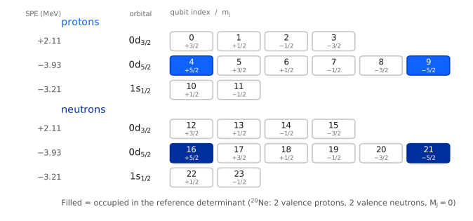
qubit แต่ละตัวคือ single-particle state แบบ $m$-scheme หนึ่งตัว $(n, \ell, j, m_j, t_z)$ และ $|1\rangle$ หมายถึง ถูกครอบครอง register ใช้ลำดับคงที่: proton ก่อน จากนั้น neutron; ภายในสปีชีส์เดียวกัน orbital ตามลำดับไฟล์; ภายใน orbital เดียวกัน $m_j$ เรียงจากมากไปน้อย ดังนั้นสองครึ่งของ bitstring จึงเป็น proton configuration และ neutron configuration นี่คือ bipartition ที่เครื่องมือ post-processing ของ pooled SQD คาดหวัง

เวิร์กโฟลว์

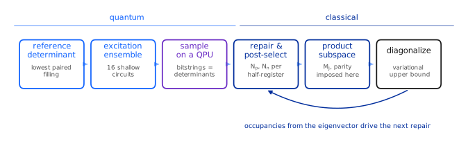
สองขั้นตอนในไดอะแกรมจัดการกับสมมาตรนิวเคลียร์

การซ่อมแซมและการคัดเลือกภายหลัง จัดการกับตัวอย่างที่ได้รับผลกระทบจาก hardware noise จำนวน nucleon ของครึ่ง register ทั้งสอง คือ Hamming weight ดังนั้น qiskit-addon-sqd จัดการกับมันโดยตรง: recover_configurations ซ่อมแซม bitstring ที่เสียหายโดยการพลิกบิตที่สอดคล้องกับค่าประมาณปัจจุบันของ occupancy orbital เฉลี่ยน้อยที่สุด แทนที่จะทิ้ง shot นั้นไป

The product subspace แนะนำ $M_J$ เนื่องจาก $M_J = M_p + M_n$ เชื่อมสองครึ่งเข้าด้วยกัน มัน ไม่ใช่คุณสมบัติของครึ่งใดครึ่งหนึ่ง ดังนั้นจึงต้องไม่ใช้เพื่อกรอง shot ทั้งหมด: bitstring ที่ครึ่ง proton และครึ่ง neutron ต่างก็ถูกต้อง ยังคงมีส่วนร่วมสอง half-configuration ที่ดีแม้ว่า $M_J$ รวมของมัน จะผิด subspace จึงถูก span โดยทุกผลคูณของ proton configuration ที่สุ่มตัวอย่างได้กับ neutron configuration ที่สุ่มตัวอย่างได้ โดยเก็บผลคูณที่ตกอยู่ใน sector $M_J$ และ parity เป้าหมาย นี่คือการสร้าง subspace แบบ pooled SQD และหมายความว่า bitstring จำนวนไม่กี่พันตัวสามารถ span subspace ที่ใหญ่กว่าจำนวนตัวอย่างมาก

สมการควบคุมสองสมการ

shell-model Hamiltonian คือเทอม one-body บวกกับปฏิสัมพันธ์ two-body

$$\begin{equation} \tag{1} H = \sum_{p} \varepsilon_p\, a_p^\dagger a_p + \tfrac{1}{4}\sum_{pqrs} \langle pq \| rs \rangle\, a_p^\dagger a_q^\dagger a_s a_r , \end{equation}$$

โดยที่ $p,q,r,s$ ระบุสถานะ $m$-scheme และ $t_z = -1$ สำหรับ proton, $+1$ สำหรับ neutron ปฏิสัมพันธ์เชิงประจักษ์ เช่น USDA [2] และ GXPF1 [3] ถูกจัดตารางไม่ใช่ใน $m$-scheme แต่ในฐาน $J$-coupled เป็น matrix element $\langle ab; J | V | cd; J \rangle$ ระหว่าง two-body state แบบ normalized antisymmetrized ของ orbital $a,b,c,d$ การกู้คืน element ของ $m$-scheme คือการ recoupling แบบ Clebsch-Gordan

$$\begin{equation} \tag{2} \langle pq \| rs \rangle = \sqrt{1 + \delta_{ab}}\sqrt{1 + \delta_{cd}} \sum_{J} \langle j_p m_p\, j_q m_q | J M \rangle \langle j_r m_r\, j_s m_s | J M \rangle \langle ab; J | V | cd; J \rangle , \end{equation}$$

โดยมีตัวประกอบ $\sqrt{1+\delta}$ ยกเลิก normalization convention ของ state ที่จัดตารางไว้ ทุกอย่างที่เหลือในบทเรียนนี้สร้างขึ้นบนสมการสองสมการนี้

การรันทั้งสามครั้ง

	นิวเคลียส	Shell	Qubit	Basis ที่สมมาตรอนุญาต	ตรวจสอบได้อย่างแม่นยำ?
ขนาดเล็ก	$^{20}\mathrm{Ne}$ (2p + 2n)	$sd$	24	640	ใช่
ขนาดใหญ่	$^{44}\mathrm{Ti}$ (2p + 2n)	$pf$	40	4,000	ใช่
ขนาดใหญ่	$^{48}\mathrm{Cr}$ (4p + 4n)	$pf$	40	1,963,461	ไม่

การรันขนาดเล็กคือ walkthrough การรันขนาดใหญ่ทั้งสองใช้ register 40 qubit: ตัวแรก ยังเล็กพอที่จะ diagonalize ได้อย่างแม่นยำบน laptop ดังนั้นคุณสามารถเปรียบเทียบผลลัพธ์ฮาร์ดแวร์กับค่าอ้างอิงที่แม่นยำได้ ตัวที่สองเกินขีดความสามารถ การทำ exact-diagonalization ของบทเรียนนี้

ทุกการรันในที่นี้ทำงานบน QPU นี่เป็นทางเลือกที่เลือกไว้สำหรับบทเรียนนี้มากกว่าจะเป็น ข้อกำหนดของวิธีการ: ทั้งสามการรันใช้ backend และ gate budget ร่วมกัน ดังนั้นคุณสามารถเปรียบเทียบประสิทธิภาพของมัน ที่ขนาดปัญหาต่างกันได้

ข้อกำหนด

ติดตั้งแพ็คเกจต่อไปนี้ก่อนเริ่มต้น:

• Qiskit SDK v2.0 ขึ้นไป (pip install qiskit)

• qiskit-ibm-runtime v0.40 or later (pip install qiskit-ibm-runtime)

• SQD addon v0.12 ขึ้นไป (pip install qiskit-addon-sqd)

• NumPy, SciPy และ Matplotlib (pip install numpy scipy matplotlib)

คุณยังต้องมีบัญชี IBM Quantum® ที่มี credential บันทึกไว้ในเครื่อง และมีสิทธิ์เข้าถึง QPU ที่มีอย่างน้อย 40 qubit

ไม่จำเป็นต้องใช้แพ็คเกจ simulator และไม่ต้องดาวน์โหลดไฟล์ข้อมูลใดๆ ไฟล์ interaction สองไฟล์ ที่บทเรียนนี้ใช้ ถูกฝังอยู่ใน setup cell ต่อไปนี้และเขียนลงในไดเรกทอรีชั่วคราวเมื่อคุณ รันมัน

การตั้งค่า

ส่วนนี้นำเข้าเครื่องมือและกำหนด shell-model helper ที่ workflow ต้องการ ตามลำดับ ที่ workflow ใช้งาน ฟิสิกส์เบื้องหลังแต่ละตัวได้มาจาก ภาคผนวก; คอมเมนต์ อธิบายบทบาทของแต่ละฟังก์ชันใน workflow

ไฟล์ interaction สองไฟล์ถูกแตกออกก่อน ทั้งสองเป็นชุดพารามิเตอร์ที่เผยแพร่แล้ว ฝังไว้ที่นี่เพื่อให้ โน้ตบุ๊กสมบูรณ์ในตัวเอง: usda.snt คือ USDA $sd$-shell Hamiltonian [2] และ gxpf1.snt คือ GXPF1 $pf$-shell Hamiltonian [3]

# Added by doQumentation — required packages for this notebook
!pip install -q matplotlib numpy qiskit qiskit-addon-sqd qiskit-ibm-runtime scipy

from __future__ import annotations

import base64
import gzip
import itertools
import tempfile
from dataclasses import dataclass
from functools import lru_cache
from math import factorial, sqrt
from pathlib import Path

import matplotlib.pyplot as plt
import numpy as np

from qiskit import QuantumCircuit
from qiskit.circuit.library import PauliEvolutionGate
from qiskit.quantum_info import Operator, SparsePauliOp
from qiskit.transpiler.preset_passmanagers import generate_preset_pass_manager
from qiskit_addon_sqd.configuration_recovery import recover_configurations
from qiskit_addon_sqd.counts import bit_array_to_arrays
from qiskit_addon_sqd.subsampling import postselect_by_hamming_right_and_left
from qiskit_ibm_runtime import QiskitRuntimeService, SamplerV2

from scipy.linalg import eigh

_USDA_SNT_GZ = (
    "H4sIAI5wqWoC/4WY224bRwyG7/UU9F0CONsZco5AUyBuC/QmQNG06KWhWGql1LYMy+kJefiOTrucGXJrQAgsf5nl8ecOr+CX"
    "D9+9g/0K9pv1/T389rx7gPLrsH+Cz/vVctg+vgAsrgB+HeDdAD9t7zYv6+dr+DDA+z8223/X17B8XMFN+ev9+m+4ed799XjA"
    "f9z8sy/4+s8BvoWYrsEERwbhFRqTXi+uCvOwW63vYf+0vFvDAgDo/AFIh8/hK7DH30354Omvb8o3V8c/vIUnMKtboK/wiGKF"
    "+gnFEfVn9PQUe8bthNIRtftbsGfUtQbAGXUFfawM8K0BF9SP6MWA0BpwQcMRvRhwBSX86+fl3ct2d4jq4+eHa3hYv2x2q7fX"
    "AJuPy+fb3cP69+Uh4luAT8djv95++eGV/fj6y6dvFudnmcX4lGOoBmttNOVncTL2FLs3NGT0l++ndJTv0cR8/t6NUanP8WMI"
    "6nPC6C8/5wp+vnn//QLOP9ank3k2wRszkDn/Zwv15xiv41l2SDmjhuEFM4PJ0QkYcgzM4A1Jp1GDkcvtaWMAR9tosAa9huHk"
    "AtoUBYwaF8hGarAxOywgxnoeN+Se2smF4H3QMPZQ653XMJpOi6GyrcLcZJtzLgoYcdsOyXKibV1Aom0fikJO0VLUMDeW3kAl"
    "qQLWpd66qGE02eZ9lXqSPD3UWyl5DeOeGnINJnmaUggCVrtgh2DJNm3fVy8WF3LSMFa9hYga5iYX0IQsYK2nmTpJkoq81Acy"
    "jLTTnPEaxqo3JGcbvZMeGnJVbw6mf2cUqcIsO80nFdOFq8JoSlY+Zb7FfNNZlnw2PqOE8SL3PtlSJhJGXGqsDRjbh4bmocWy"
    "oiIxSxjv09JYgaxlGLZxA9EFFOImuIBt3EB04TK3Z5S8wizrrFCJQ4Xpgl9hzDYbu0LCNm6HzkJHweUkYazITalyF7NjGAnh"
    "FZJFQniFZFHnqWgbdZ6qtoX50VZhvEJ81TJe7AUcQozH8yQMJ8ymUS07jLin6LXT3FRIhmwSTmtbJpEjr2AsvM7E1ra+ZaiM"
    "NoxewZinBlPQTmPJyikn7TQ2630SbWuz4CLlwzuGhCHPqbUmRZQwpkiBDn1vsoQ55oKjbEvNNVgbXls0WvA0NKnPpku91Fkx"
    "pahhXPDJtxVCQkBcMtJD27I8VJGAhWYYlVuZzc5e+jSIZWnLa57nOQ1iWZY+jSE3GP5/QIKi5E1Agqi9BbMZiUjEWNwChqKq"
    "KTZY11ku5ca2Pqc4YKk1o2DstBjJC1htW2nAgEZ4aDdPvQmmmLeY4tWFt9Y3VAdlpW+oDcpa3zpM1jdUB2XV9agOyqrrcWZQ"
    "sq7vMMffBseux5l5yjoLZ+Yp6yzU5mmt5DgzT5mSozZPoVIknJmnTJFQHZRV12OrlvpFQFbycoGKOWiYfl9QlXySGtSUvL9W"
    "VJi/YG4grC4CmuCX6CZrKUsY64UyJolCQoZJqWeKhDOCzxQJNcGXbZMEX7EtzF+gvCI1npxjmKaW5Q06ewVjOY0u2+Y0kt5D"
    "JhlETS2P+5CqyIMYkCI1NK50SO3TarSR2qfVaKOZPmXjg2beVJmS01zqp/CSmvoqvNSOD/kaS+qUoSGaTM2yz83fdjtMvsZy"
    "xOv7N44Fff/GT5q5tXWYfB3jWND3b9yumUvK5SQnvK6w/VuHyfu3DpP3bx0m7984FvT9W4fJ+zceWq/v3zpM3r9xLOj7tw6T"
    "928X053QgGz/1mHy/u3yZ8lTtn/jWND3b74NiDx2vRbeep56Lbz1oPRaeOv9G0dmxofXPK33bx0m798C1B9RuP4DPJ0WcLAa"
    "AAA="
)

_GXPF1_SNT_GZ = (
    "H4sIAI5wqWoC/4WcQY8dtw3H7/kU41sCeF8lUqKkQw9NgbaXoEHQQ26BkdiIEWdt2E6L9tNXb9+ORIn8PwdZILB/S3I4IsW/"
    "ZiYvjr//+P3f4nG8ef/x+PDm4dOvr9+9++rF8d3l+Mf7x99fvTz+dTn++fnTH7/1//z28pfL8e3H9/95fHm8evzl+lffvf3f"
    "H59e/fb26L9zHN//+t9Pl+OH1/++HH89JL88gkQO8esfvjm+phDomyvW//39/S+v3x2fPrz6+fVX/dfS889B4fpz/aN43P7p"
    "f3Bw/ynH8fD0Zy+uf/fn48MR3vxU/kRXlp7Z+PzDiqUnNn74iW8sb3azYvm0m29s2uxGxabTbryx2cZ7nGzu7KOKV2y8g5Un"
    "dsZbbLyDLafd53irjXew9bR7jffF8fbx8+uPr37+/Pb941dPv3P93ZH4W/If6kUohXCm+Jbmh3yR0jicybwl9CFeuFILy908"
    "HtIlcrlZyCNJ2q6MdGi7ZVy4tlvHJS52Y71FnHp8D+HCIYTlQuYFhdsv0yVxzZB6vsxwaZwJUumkIjWB1POdDhcqlR2KVo85"
    "SoDU8NgdNodiZevqMUqB1LCVWsO2ZMQlyYs+bXEFk4m5bMJJlVgSpGjaouhQvFKxUIbUjIvI85hWW4FNvubyDnMxMkFKRc8V"
    "Uml65OhQW1x9fe3XOAtsZPXJ36TIX18SaoQUnysnZsHUXPfcKqTyaSu36FHbWg0tN0jxWIXEAVLzbqcqkMpj3T8lwlBp9RhD"
    "qpAaHpnzni9nRXPh6lDbysmJBVLzDtU71KztnDxqW1+JhDaKnTtUa4DUzH00Hp0VXQMHSM3c16irlpf7GEcN1dogpfpEDpAa"
    "WRUOBKl0UqkIQ2qs+5IYU6OvthbFodIaF6/9i51VeF0TLZSN2lfh9T729utQOqtXKi/dl/21mihhW+M+BpIKqblypDWHSntc"
    "mSA1O3nMe+6dHp0DEaRmXCU0h9p7dOYCqVm1MehOnvy7nWphSKnuu+Q++X2Ca4uQGrYkxp3yMkFLL0ygavPovmR64dhFY5QM"
    "KVK1XRxqX4UydlHCXU44hY1ydndKuUBK11BzqH1NNOKNMvt27PMXVUWBemSqCVIjrr4nYFtzTSQJkJp3O7se09p9YygCKVL7"
    "UN4opx5DNnE5q5AlerZ2jyExpEYmggTtMYFrzC1Bak58jetGeSvHenSip9ROik0m5lqdsxzjrCYhTM1uImOHYZzVPvnWjXIm"
    "0RoaKyqhjjlqiEE3uWoYHqopbT/KY0pDD+Xtx9d8lvI0n6U8zWcpT/NpQqDms5Sn+TRVoOazlKf5LOVpPk1VqPl05AI1n6U8"
    "zaepAjWfpTzNp6kKNZ/OQoGaz1Ke5rOUp/k0VaHm03mvUPOd1+esL6X5LOVpPkt5ms9SnubTVIGaz1Ke5rOUp/ks5Wk+TVWo"
    "+SzlaT69mgVqPk0VqPks5Wk+S3maT1MVaj5dPwVqPkt5mk9TFWo+S3ma77x/8z56ms9SnuazlKf5LOVpPkt5ms9SnubTVIWa"
    "z1Ke5jupfRWumk9TBWo+S3maz1Ke5rOUp/k0VaHms5Sn+XTnLVDzWcrTfJqqUPNZytN85/1z7rbSfJbyNN/5t06fUJrPUp7m"
    "OykvE7T0wgqqdmo+Mb3Q03yCO6bSfII7ptJ8gruc0nxi+pen+eROL5yaT3CXU5pPx1Sh5hNcj0rzCajHVfMJqMdV88mdesyu"
    "xwo1n+B6VJpPcD0qzSe4HpXmE1yPSvMJrkelwERVR4Waz1Ke5hNTQ3THoxO90nzFZMLTfAVnVWm+grOqNF/BWVWaTxMVar6C"
    "r1FpvgK6yar56vbja76onormu8/5ViqOrNblZH6l0NPAlRq9sKaIbaFnhis15tUuH/E1oieLK1XOTIgsz3ROap9XpQ/SJWqK"
    "bCYcKm6K4tp9iUqqzbd1j4qO+g2tpTV6sll1qLipk6fnw32/isDWPSruPborwz7x9eakKbbry6Gi7RN9nrhuHr4tPXXsVLT9"
    "vvTdKlUQ18i9Q0Wn+2ZOlYpva0yiDhXthNz69p4S+7ZG7h0q2jma+/BIIfm2RnU4VLQ9R6hG4iWryVurhorOlNbzEJr4tubk"
    "bim6e25iqbFbJY4MKfREfaXGNXKK2aF2BSapD6Oy5162yd1S5Og0iq3k5tua1WEpsus+ZO4ZS76tqU4sRc7+mAtJyL6teR8t"
    "RVbDUO9yXM2a2O6jQ5GjdCi3HKpva04dluK7J1uWGtFLjhFS6J2HlZpKhzOm0JsRK5XnmjD7Izv5av0eBd7zVb5IsVU6ffTN"
    "oQXf1peoeveNjZWaNURFZ0L8fTsX1s9hwO4eeHkOA3Z3Zct6ZOccgPAM0O91hR4ZPEcWMAPkdBWQvsdZj72xZuTRs2U95qFY"
    "a8FZHVQpy/Mhd55YbGmPew2VGB2PRvOVsNlib0orYbO1U8fi0cbF6uQhw7jUycMybYs/dSiKwGxyLB5tXEmdM5WM4lKnGLFm"
    "FFeaPTruK8ehlEcbV55n2yIwrnlOXorAuPKsxyIwrjz7l3greptzSgve+tqo2lLbcu9MQ4oiPDMpjzaueR8rUUZxqaql/T46"
    "k5WiCM9fyuNpy5uZpM9WkvfaxpS1Ndd96JKV2LflUdrW1idaKOT0HNMnTCdnT/OZvcOZv5RHG5fqAJFhXLO2WykwrtlzJkV4"
    "llMebVxp7kOUMopr7h1dSmcUl9LuxesT2z6kPOq4ttkkk7sj1/1JWWWnHvfdfVKE50LlUV+jObPqs2hO+zViytpSJ+CFSyu+"
    "LY+yttRM3gf3HH1bHmVtzR5NXZQXcI0epW1tdyh2d86a2O52F9vR6V8FUgTm1dWjjWuepZUgMK45k2cKMC6PIjD7rh6j+gpi"
    "0Y904b675/n2h3u6QteTedkoc7qy2LIeaUxpkXNAHgeV53khozOYxZb1qDpTrvAa+TxBClECvEbPlvWY5o4cA7zGNDSfFIbX"
    "6NmyHmd1SEnwGgfVJ6YKr9GzZT3KebdDZIYe5bzGQLFAj54t7XHXfDkmJ6v789r17e7iTEMrxXhmUh5tXHNmainCuObMVBOO"
    "y6MYzEyrx9MW2VMf4cC9NWlbzpmVoqytucPkIO12SsZ4/lKUtTX7V6LGsfi2phadlLa1nX89naUHc437uYnQni/nlEzWN/S8"
    "s7TVo41LvUsW9+pwqFBl79HsPYkVr/sK9GjjYnVWSzBfqjoowXx5FN+ZC6dHG5d6WybjfM15ouYE8+VRDObC1aOOa3v+WEJq"
    "Tlzb2VCRELOtbYEU47NH5dHGpd5nagzj0s+HAozLoxjMq6tHnfutHmNjblz23G/1qChra3rMOT6f3jGefRVlbamZKfR1COKa"
    "PWdS1tZcXy3mnMm3pd4IGpS1Nd9Uai0Wir6t+fxxUtrWPvu27M1MG8XJ1KMz+yqK8Vmt8mjjmn1CKmcUF88zhVIzimtOtZNi"
    "fO6rPGpbW9XGLrg50G5rfwNhUueu7swmEtI55yQ0m/RpqI3JPd15ujVtWY9TSbcxpSU8dSShAj16tk4b3r6dmUlI2/L27Ulp"
    "W7vKLFK3uByK4nI2VP19SFEJ7EOrRxvXyESr413YhPchLsssV/0dRlEJ70PKo7a1n/vWa1rLbsu8mTooa0up8tpyEd+Wep42"
    "KG1rf6su5ebkvpqztLzl3qltRSVc28ojmTM+9F2TwNm3Qgp9/eSeKnaNXFtwqH3nk1KaJE05M6ZDOdNjv9NJIvm2Zr+3lFeP"
    "EvqGnH1bM/eWMtNQvFCRHnzUlJlzXMqZYFKqHHLxbdFUFIbiu+8XWmo+50vL6R06l1u/PBO/asN8B5zAmdXTDtP7r8h+jeWL"
    "lFOPocYumti39SWq3v0iTvxdtDw9hhmUq9N6PbaqvzJyqyNeMi0nIm51LLbojgIrOUKP+l2yBj16tghrqxib1gqg0pLknfIq"
    "bdoirJqkMMNrnDNATPgaPVuE9VBv0J7HbU107V42W44eUhSjPrF4JKyHUokZxqXeTV+exAI9pCjGp/zKIwE9dO2+XSTX1vbc"
    "b6pJUYT1UOCWWw2+rdmZJkVYD1Ef0Uoi39acySdFWA9RztLVjm9LPQ0cFAENc3unJjrVsWuY0mK297EYxbrbcs7vlUfCGib3"
    "bQ/GNWffMijCGkZRDHr0w+KRsIbpnem6dnZbe9VOitTsW7e3I+e7Pgnv7tfHQxvl7O7KlvU4zu95fouUUNV21RSGFk2oHhdb"
    "ZGbf+b4cXf8nRlnb8maASVlbc+UkSnSb0hKox4eFIjNHz7c/aHydkvC6T9Lydo3Je+u8ZSdf+xsu06O2ta2vPr70W1l2W9v6"
    "UhSbPoG+kwYnSDVnTKGvqYvfv3JuDVLom2vvpOZpvh9fizHuX71jVp79vqDcG8rrJolLnecTxe8TgMLfBTDoJteOGUVntYJr"
    "5PHOVsKnUaEuJw8oE9MWA5V5e2tA9wmQrw5xQB6RrernS33VkEB1PCmKW5f7P6zudeW7TwAA"
)

DATA = Path(tempfile.mkdtemp(prefix="nuclear_sqd_"))
for name, blob in (("usda.snt", _USDA_SNT_GZ), ("gxpf1.snt", _GXPF1_SNT_GZ)):
    (DATA / name).write_bytes(gzip.decompress(base64.b64decode(blob)))

    if not (DATA / name).is_file():
        raise RuntimeError(f"{name} did not unpack to {DATA}")

พื้นที่แบบจำลองและเรจิสเตอร์ Qubit

ไฟล์ .snt เก็บพื้นที่แบบจำลอง พลังงาน single-particle และ matrix element แบบ two-body ที่ $J$-coupled สำหรับปฏิสัมพันธ์ที่ขึ้นกับมวลที่ใช้ในที่นี้ field ที่สามและสี่ของส่วนหัว two-body ระบุมวลอ้างอิง $A_{\mathrm{ref}}$ ที่ปฏิสัมพันธ์ถูก fit ไว้ และเลขชี้กำลังของการขึ้นกับมวลของมัน ทั้งสอง ไฟล์มีเลขชี้กำลัง $-0.3$ โดยมี $A_{\mathrm{ref}} = 18$ สำหรับ USDA และ $42$ สำหรับ GXPF1 ดังนั้น matrix element ที่จัดตารางไว้ต้องถูกปรับขนาดใหม่ด้วย $(A/A_{\mathrm{ref}})^{-0.3}$ สำหรับนิวเคลียส ที่กำลังคำนวณ [2], [3] พลังงาน single-particle ไม่ถูกปรับขนาดใหม่ การข้าม ขั้นตอนนี้เปลี่ยนพลังงาน correlation ไปไม่กี่เปอร์เซ็นต์

พลังงานที่ตามมาคือพลังงาน valence วัดจาก core เฉื่อย ไม่ใช่พลังงาน separation เชิงทดลอง

@dataclass(frozen=True)
class Orbital:
    idx: int
    n: int
    ell: int
    j2: int
    tz: int  # j2 = 2j; tz = -1 proton, +1 neutron

@dataclass(frozen=True)
class SPState:
    """One m-scheme single-particle state, i.e. one qubit."""

    orb: int
    j2: int
    mj2: int
    tz: int
    ell: int
    spe: float  # mj2 = 2 * m_j

@dataclass
class ModelSpace:
    orbitals: list
    spes: dict
    tbmes: dict
    core_z: int
    core_n: int
    mass_number: int
    a_ref: int
    mass_exponent: float
    mass_factor: float

def read_snt(path, n_protons, n_neutrons):
    """Parse a .snt interaction file, applying its mass dependence for this nucleus.

    The two-body header line is ``n_tbme  method  A_ref  exponent``.  When ``method`` is 1 the
    tabulated matrix elements are rescaled by ``(A / A_ref) ** exponent``, where A is the mass
    number of the whole nucleus -- the core plus the valence nucleons.  A is derived from the
    file's own core numbers rather than passed in, so it cannot silently disagree with the
    valence counts the rest of the workflow uses.  Single-particle energies are not rescaled.
    """
    rows = [
        ln.split("!")[0].split() for ln in Path(path).read_text().splitlines()
    ]
    rows = iter([r for r in rows if r])

    n_p_orb, n_n_orb, core_z, core_n = (int(x) for x in next(rows)[:4])
    orbitals = [
        Orbital(*(int(x) for x in next(rows)[:5]))
        for _ in range(n_p_orb + n_n_orb)
    ]

    spes = {}
    for _ in range(int(next(rows)[0])):  # "i  i  <i|H(1b)|i>"
        field = next(rows)
        spes[int(field[0])] = float(field[2])

    n_tbme, method, a_ref, exponent = next(rows)[:4]
    n_tbme, method, a_ref, exponent = (
        int(n_tbme),
        int(method),
        int(a_ref),
        float(exponent),
    )
    mass_number = core_z + core_n + n_protons + n_neutrons
    factor = (mass_number / a_ref) ** exponent if method == 1 else 1.0

    tbmes = {}
    for _ in range(n_tbme):  # "a  b  c  d  J  value"
        field = next(rows)
        tbmes[tuple(int(x) for x in field[:5])] = float(field[5]) * factor

    return ModelSpace(
        orbitals,
        spes,
        tbmes,
        core_z,
        core_n,
        mass_number,
        a_ref,
        exponent,
        factor,
    )

def m_scheme_states(ms):
    """The qubit register: protons then neutrons, orbitals in file order, m_j descending."""
    return [
        SPState(o.idx, o.j2, m2, o.tz, o.ell, ms.spes[o.idx])
        for tz in (-1, +1)
        for o in ms.orbitals
        if o.tz == tz
        for m2 in range(o.j2, -o.j2 - 1, -2)
    ]

การจับคู่ใหม่แบบ Clebsch-Gordan

สมการ (2) ต้องการสัมประสิทธิ์ Clebsch-Gordan สำหรับโมเมนตัมเชิงมุมแบบครึ่งจำนวนเต็ม ทุกอาร์กิวเมนต์ถูก ส่งเป็น สองเท่า ของค่าทางกายภาพ ดังนั้น $j = 5/2$ จึงเข้าเป็น 5 และเลขคณิตยังคงแม่นยำ

Interaction.v_ms จัดการการค้นหา matrix element ของ interaction ไฟล์ .snt เก็บแต่ละ matrix element ไว้เพียงครั้งเดียว ดังนั้นการค้นหาอาจต้องใช้เฟส pair-exchange แบบ antisymmetrized $-(-1)^{j_a + j_b - J}$ ด้าน ใดด้านหนึ่ง และ bra กับ ket อาจถูกเก็บไว้ในลำดับใดก็ได้

@lru_cache(maxsize=None)
def clebsch_gordan(j1_2, j2_2, J_2, m1_2, m2_2, M_2):
    """<j1 m1 j2 m2 | J M>.  Every argument is twice its physical value."""
    if m1_2 + m2_2 != M_2 or not abs(j1_2 - j2_2) <= J_2 <= j1_2 + j2_2:
        return 0.0
    if abs(m1_2) > j1_2 or abs(m2_2) > j2_2 or abs(M_2) > J_2:
        return 0.0
    if (j1_2 + j2_2 - J_2) % 2 or (j1_2 - m1_2) % 2 or (j2_2 - m2_2) % 2:
        return 0.0

    f, half = factorial, lambda x: x // 2
    prefactor = sqrt(
        (J_2 + 1)
        * f(half(j1_2 + j2_2 - J_2))
        * f(half(j1_2 - j2_2 + J_2))
        * f(half(-j1_2 + j2_2 + J_2))
        / f(half(j1_2 + j2_2 + J_2) + 1)
        * f(half(J_2 + M_2))
        * f(half(J_2 - M_2))
        * f(half(j1_2 - m1_2))
        * f(half(j1_2 + m1_2))
        * f(half(j2_2 - m2_2))
        * f(half(j2_2 + m2_2))
    )
    total = 0.0
    for k in range(half(j1_2 + j2_2 - J_2) + 1):
        d = [
            half(j1_2 + j2_2 - J_2) - k,
            half(j1_2 - m1_2) - k,
            half(j2_2 + m2_2) - k,
            half(J_2 - j2_2 + m1_2) + k,
            half(J_2 - j1_2 - m2_2) + k,
        ]
        if all(x >= 0 for x in d):
            total += (-1) ** k / (
                f(k) * f(d[0]) * f(d[1]) * f(d[2]) * f(d[3]) * f(d[4])
            )
    return prefactor * total

class Interaction:
    """Antisymmetrized m-scheme two-body matrix elements <pq||rs>, per Eq. (2)."""

    def __init__(self, model_space, sp):
        self.ms, self.sp, self._cache = model_space, sp, {}

    def _tbme(self, oa, ob, oc, od, J, j_ab_2, j_cd_2):
        """<oa ob; J|V|oc od; J>, allowing for how the file happens to order each pair."""
        table = self.ms.tbmes
        # |ba; J> = -(-1)^(j_a + j_b - J) |ab; J> for a normalized antisymmetrized pair;
        # dropping the leading minus makes v_ms symmetric instead of antisymmetric, and
        # the Hamiltonian then fails the rotational-invariance check in Step 1.
        phase_ab = -1.0 if (j_ab_2 // 2 - J) % 2 == 0 else 1.0
        phase_cd = -1.0 if (j_cd_2 // 2 - J) % 2 == 0 else 1.0
        for keys, phase in (
            (((oa, ob, oc, od), (oc, od, oa, ob)), 1.0),
            (((ob, oa, oc, od), (oc, od, ob, oa)), phase_ab),
            (((oa, ob, od, oc), (od, oc, oa, ob)), phase_cd),
            (((ob, oa, od, oc), (od, oc, ob, oa)), phase_ab * phase_cd),
        ):
            for key in keys:
                value = table.get(key + (J,))
                if value is not None:
                    return value * phase
        return 0.0

    def v_ms(self, p, q, r, s):
        """<pq||rs>, zero unless M_J and charge are conserved."""
        cached = self._cache.get((p, q, r, s))
        if cached is not None:
            return cached

        P, Q, R, S = (self.sp[i] for i in (p, q, r, s))
        value = 0.0
        if P.mj2 + Q.mj2 == R.mj2 + S.mj2 and P.tz + Q.tz == R.tz + S.tz:
            M = P.mj2 + Q.mj2
            # sqrt(1 + delta): undo the normalization of the tabulated pair states
            c12 = sqrt(2.0) if (P.tz == Q.tz and P.orb == Q.orb) else 1.0
            c34 = sqrt(2.0) if (R.tz == S.tz and R.orb == S.orb) else 1.0
            for J2 in range(
                max(abs(P.j2 - Q.j2), abs(R.j2 - S.j2)),
                min(P.j2 + Q.j2, R.j2 + S.j2) + 1,
                2,
            ):
                cg_bra = clebsch_gordan(P.j2, Q.j2, J2, P.mj2, Q.mj2, M)
                cg_ket = clebsch_gordan(R.j2, S.j2, J2, R.mj2, S.mj2, M)
                if abs(cg_bra) < 1e-12 or abs(cg_ket) < 1e-12:
                    continue
                value += (
                    c12
                    * c34
                    * cg_bra
                    * cg_ket
                    * self._tbme(
                        P.orb,
                        Q.orb,
                        R.orb,
                        S.orb,
                        J2 // 2,
                        P.j2 + Q.j2,
                        R.j2 + S.j2,
                    )
                )

        self._cache[(p, q, r, s)] = value
        return value

องค์ประกอบเมทริกซ์และการทดสอบสมมาตร

determinant คือ tuple ที่เรียงลำดับของดัชนี qubit ที่ถูกครอบครอง determinant สองตัวที่ต่างกันในสถานะที่ถูกครอบครองมากกว่า สองสถานะ มี matrix element เป็นศูนย์ มิฉะนั้น กฎ Slater-Condon จะให้ผลรวมสั้นๆ เหนือ interaction คูณด้วยเครื่องหมาย fermionic ที่นับว่ามีสถานะที่ถูกครอบครองกี่สถานะอยู่ระหว่าง ตัวดำเนินการในลำดับ register คงที่

symmetry_allowed คือการทดสอบจำนวนเต็มที่เลขควอนตัมที่แน่นอนทั้งสี่ตัวลดรูปลงมา มันถูกใช้ทั้ง เพื่อกรองตัวอย่างและเพื่อระบุ basis ที่แม่นยำสำหรับการรันที่เล็กพอจะตรวจสอบได้

def matrix_element(inter, det_a, det_b):
    """<A|H|B> for two determinants, each a sorted tuple of occupied qubit indices."""
    set_a, set_b = set(det_a), set(det_b)
    out_a, out_b = sorted(set_a - set_b), sorted(set_b - set_a)
    if len(out_a) != len(out_b) or len(out_a) > 2:
        return 0.0

    if not out_a:  # diagonal: one-body plus two-body
        return sum(inter.sp[i].spe for i in det_a) + sum(
            inter.v_ms(i, j, i, j)
            for i, j in itertools.combinations(det_a, 2)
        )

    if len(out_a) == 1:  # one state moves, p -> q
        p, q = out_a[0], out_b[0]
        crossings = sum(1 for k in set_a if min(p, q) < k < max(p, q))
        return (-1.0) ** crossings * sum(
            inter.v_ms(p, j, q, j) for j in det_a if j not in (p, q)
        )

    (p, r), (q, s) = out_a, out_b  # two states move
    crossings = sum(1 for k in set_a if p < k < r) + sum(
        1 for k in set_b if q < k < s
    )
    return (-1.0) ** crossings * inter.v_ms(p, r, q, s)

def subspace_hamiltonian(inter, dets):
    """Dense real-symmetric H projected onto the span of `dets`."""
    H = np.zeros((len(dets), len(dets)))
    for a, det_a in enumerate(dets):
        H[a, a] = matrix_element(inter, det_a, det_a)
        for b in range(a + 1, len(dets)):
            H[a, b] = H[b, a] = matrix_element(inter, det_a, dets[b])
    return H

def ground_state(inter, dets):
    """Lowest eigenvalue and eigenvector of H over `dets`."""
    values, vectors = np.linalg.eigh(subspace_hamiltonian(inter, dets))
    return values[0], vectors[:, 0]

def symmetry_allowed(
    sp, det, n_protons, n_neutrons, mj2_target=0, parity_target=0
):
    """The four exact shell-model quantum numbers, as integer tests on one determinant."""
    n_p = sum(1 for i in det if sp[i].tz == -1)
    return (
        n_p == n_protons
        and len(det) - n_p == n_neutrons
        and sum(sp[i].mj2 for i in det) == mj2_target
        and sum(sp[i].ell for i in det) % 2 == parity_target
    )

def full_basis(sp, n_protons, n_neutrons, **targets):
    """Every symmetry-allowed determinant.  Only tractable for small model spaces."""
    protons = [i for i, s in enumerate(sp) if s.tz == -1]
    neutrons = [i for i, s in enumerate(sp) if s.tz == +1]
    return [
        p + n
        for p in itertools.combinations(protons, n_protons)
        for n in itertools.combinations(neutrons, n_neutrons)
        if symmetry_allowed(sp, p + n, n_protons, n_neutrons, **targets)
    ]

def count_basis(sp, n_protons, n_neutrons, mj2_target=0, parity_target=0):
    """How many determinants `full_basis` would return, without enumerating them.

    A dynamic program over (occupied count, sum of 2*m_j, parity) per species.  This stays
    cheap when the basis itself is far too large to build, which is how the largest run below
    can report the size of the space it is sampling from.
    """

    def species(states, k):
        table = {(0, 0, 0): 1}
        for s in states:
            for key, value in list(table.items()):
                count, m_sum, parity = key
                if count < k:
                    nxt = (count + 1, m_sum + s.mj2, (parity + s.ell) % 2)
                    table[nxt] = table.get(nxt, 0) + value
        totals = {}
        for (count, m_sum, parity), value in table.items():
            if count == k:
                totals[(m_sum, parity)] = (
                    totals.get((m_sum, parity), 0) + value
                )
        return totals

    left = species([s for s in sp if s.tz == -1], n_protons)
    right = species([s for s in sp if s.tz == +1], n_neutrons)
    return sum(
        a * b
        for (mp, pp), a in left.items()
        for (mn, pn), b in right.items()
        if mp + mn == mj2_target and (pp + pn) % 2 == parity_target
    )

ดีเทอร์มิแนนต์อ้างอิง

ansatz ถูกสร้างขึ้นบน determinant เดียว ดังนั้น determinant นั้นควรเป็นตัวที่ดีที่สุดที่มี อยู่ การเติมพลังงาน single-particle ที่ต่ำที่สุดจะไม่สนใจปฏิสัมพันธ์ two-body ในพื้นที่แบบจำลองเหล่านี้ ตัวเลือกนั้นให้พลังงานสูงกว่า determinant ที่มีพลังงานต่ำที่สุด 1-2 MeV

การจำกัดให้เป็นการเติมที่ประกอบด้วยคู่ time-reversed $(+m_j, -m_j)$ บังคับให้ $M_J = 0$ อย่างแม่นยำ และเหลือเพียง $\binom{n_{\mathrm{pairs}}}{k}$ ตัวเลือกต่อสปีชีส์ (มากที่สุดไม่กี่พันตัว) ดังนั้น ตัวที่ดีที่สุดสามารถหาได้โดยค้นหาทั้งหมดบน diagonal เต็ม $\langle \Phi | H | \Phi \rangle$ กรณีเสมอกันจะตกเป็นของคู่ที่จัดเรียงกันแน่นที่สุด ซึ่งเป็นจุดที่แรง pairing $J = 0$ แข็งแกร่งที่สุด ในทุก กรณีในบทเรียนนี้ที่สามารถตรวจสอบกับการนับทั้งหมดได้ การค้นหาคืนค่า determinant ที่มี diagonal ต่ำที่สุดทั่วโลก ซึ่งเป็นองค์ประกอบเดี่ยวที่ใหญ่ที่สุดของสถานะพื้นที่แม่นยำด้วย

def reference_determinant(sp, inter, n_protons, n_neutrons):
    """Lowest-diagonal determinant built from time-reversed (+m_j, -m_j) orbital pairs."""
    if n_protons % 2 or n_neutrons % 2:
        raise ValueError(
            "an odd valence count has no time-reversed paired reference at M_J = 0"
        )

    def species_pairs(tz):
        return [
            (
                q,
                next(
                    p
                    for p, t in enumerate(sp)
                    if t.tz == tz and t.orb == s.orb and t.mj2 == -s.mj2
                ),
            )
            for q, s in enumerate(sp)
            if s.tz == tz and s.mj2 > 0
        ]

    best = None
    for chosen_p in itertools.combinations(species_pairs(-1), n_protons // 2):
        protons = tuple(q for pair in chosen_p for q in pair)
        for chosen_n in itertools.combinations(
            species_pairs(+1), n_neutrons // 2
        ):
            det = tuple(
                sorted(protons + tuple(q for pair in chosen_n for q in pair))
            )
            # break ties toward the most aligned pairs, where J = 0 pairing is strongest
            score = (
                matrix_element(inter, det, det),
                -sum(abs(sp[q].mj2) for q in det),
            )
            if best is None or score < best[0]:
                best = (score, det)
    return best[1]

กลุ่มการกระตุ้นและการจัดลำดับเชิงเพอร์เทอร์เบชัน

Correlation ถูกนำพาโดย excitation แบบ two-particle–two-hole ($2p2h$) จาก reference กฎการคัดเลือก สองข้อลดจำนวน pool ก่อนที่จะสร้างวงจรใดๆ: excitation ต้องอนุรักษ์ $M_J$ และคู่ hole กับคู่ particle ต้อง coupling กับ $J$ รวมร่วมกันได้ ซึ่งเป็น triangle inequality

excitation ที่เหลือถูกจัดอันดับตามคะแนน Epstein-Nesbet อันดับสองของ selected configuration interaction [4]

$$\begin{equation} \tag{3} s_\alpha = \frac{|\langle \Phi_{\mathrm{ref}} | H | \alpha \rangle|^2}{|\Delta_\alpha|}, \qquad \Delta_\alpha = H_{\mathrm{ref},\mathrm{ref}} - H_{\alpha\alpha}, \end{equation}$$

ซึ่งประมาณว่าแต่ละ excitation นำพาพลังงาน correlation เท่าใด ตัวเลขสองตัวเดียวกันนี้กำหนด มุมของวงจร: ด้วย $V = \langle \Phi_{\mathrm{ref}} | H | \alpha \rangle$ แอมพลิจูดอันดับหนึ่ง คือ $t_\alpha = V / \Delta_\alpha$ ภาคผนวก อธิบายว่าทำไมแอมพลิจูดอันดับหนึ่งจึงเป็น ตัวเลือกที่ใช้ในบทเรียนนี้แทนที่จะเป็นมุม two-level ที่แม่นยำ

def excitation_pool(sp, occ):
    """2p2h quadruples (h1, h2, v1, v2): same-species pairs, then proton-neutron pairs."""
    holes = {tz: [i for i in occ if sp[i].tz == tz] for tz in (-1, +1)}
    virtuals = {
        tz: [i for i, s in enumerate(sp) if s.tz == tz and i not in occ]
        for tz in (-1, +1)
    }
    pool = [
        (h1, h2, v1, v2)
        for tz in (-1, +1)
        for h1, h2 in itertools.combinations(holes[tz], 2)
        for v1, v2 in itertools.combinations(virtuals[tz], 2)
    ]
    pool += [
        (h1, h2, v1, v2)
        for h1 in holes[-1]
        for h2 in holes[+1]
        for v1 in virtuals[-1]
        for v2 in virtuals[+1]
    ]
    return pool

def conserves_symmetry(sp, op):
    """Keeps M_J, and the hole and particle pairs share a reachable total J."""
    h1, h2, v1, v2 = op
    if sp[v1].mj2 + sp[v2].mj2 != sp[h1].mj2 + sp[h2].mj2:
        return False
    return max(abs(sp[v1].j2 - sp[v2].j2), abs(sp[h1].j2 - sp[h2].j2)) <= min(
        sp[v1].j2 + sp[v2].j2, sp[h1].j2 + sp[h2].j2
    )

def en_denominator(inter, occ, holes, virtuals, floor=0.1):
    """Epstein-Nesbet gap: bare gap, spectator rearrangement, and the pair's own term."""
    gap = sum(inter.sp[h].spe for h in holes) - sum(
        inter.sp[v].spe for v in virtuals
    )
    for k in occ:
        if k in holes:
            continue
        gap += sum(inter.v_ms(h, k, h, k) for h in holes)
        gap -= sum(inter.v_ms(v, k, v, k) for v in virtuals)
    gap += inter.v_ms(holes[0], holes[1], holes[0], holes[1])
    gap -= inter.v_ms(virtuals[0], virtuals[1], virtuals[0], virtuals[1])
    return gap if abs(gap) >= floor else (floor if gap >= 0 else -floor)

def rank_pool(inter, occ, pool):
    """Sort by descending PT2 score; return (operator, coupling, first-order amplitude)."""
    ranked = []
    for op in pool:
        h1, h2, v1, v2 = op
        coupling = inter.v_ms(v1, v2, h1, h2)
        gap = en_denominator(inter, occ, (h1, h2), (v1, v2))
        ranked.append((coupling**2 / abs(gap), op, coupling, coupling / gap))
    ranked.sort(key=lambda row: (-row[0], row[1]))  # deterministic on ties
    return [
        (op, coupling, amplitude) for _, op, coupling, amplitude in ranked
    ]

บล็อกการกระตุ้นแบบ Qubit

ภายใต้การ mapping แบบ Jordan-Wigner ตัวดำเนินการ excitation แบบ $2p2h$ ที่อนุรักษ์ particle จะกลายเป็นผลรวมของ Pauli string แปดตัว แต่ละตัวมีสาย $Z$ operator ระหว่างดัชนีนอกสุด สาย $Z$ บังคับ fermionic antisymmetry และมันมีราคาแพง: excitation แบบ proton-neutron ขยายผ่านขอบเขตระหว่างสองครึ่งของ register และรวมสาย parity ข้ามขอบเขตนั้นด้วย

การตัดสาย $Z$ ออกจะให้ตัวดำเนินการ qubit-excitation ของ Yordanov et al. [5] สถานะที่เตรียมโดยตัวดำเนินการนี้มีแอมพลิจูดต่างกัน แต่มันเชื่อมต่อคู่ determinant เดียวกันทุกประการ ดังนั้นชุดของ determinant ที่วงจรสามารถ ไปถึงได้จึงไม่เปลี่ยนแปลง pooled SQD ใช้ determinant เหล่านี้สำหรับ classical diagonalization ขั้นตอนที่ 2 เปรียบเทียบ support ของทั้งสองโครงสร้างและวัดต้นทุนฮาร์ดแวร์ของพวกมัน

การสร้างรูปแบบ Pauli จาก $a_j^\dagger = \tfrac{1}{2}(X_j - i Y_j) \otimes Z_{<j}$ โดยที่สาย $Z$ เป็นตัวเลือก ทำให้ทั้งสองโครงสร้างต่างกันเพียง flag เดียว ทั้งแปดเทอมของ generator เดียวกัน commute กัน ดังนั้นขั้นตอน PauliEvolutionGate เดียวจึงเป็น exponential ที่แม่นยำ ไม่ใช่การประมาณแบบ Trotter ต่อมัน

def _ladder(num_qubits, q, dagger, parity):
    """Pauli form of a_q or a_q^dagger.  `parity` toggles the Jordan-Wigner Z string."""
    prefix = (
        ["Z"] * q + ["I"] * (num_qubits - q) if parity else ["I"] * num_qubits
    )
    x_part, y_part = list(prefix), list(prefix)
    x_part[q], y_part[q] = "X", "Y"
    return SparsePauliOp(
        ["".join(reversed(x_part)), "".join(reversed(y_part))],
        coeffs=[0.5, 0.5 * (-1j if dagger else 1j)],
    )

def excitation_generator(num_qubits, op, parity=False):
    """Hermitian H with exp(-i theta H) = exp(theta (T - T^dagger)) for T = a+ a+ a a."""
    h1, h2, v1, v2 = op
    T = SparsePauliOp("I" * num_qubits)
    for q, dagger in ((v1, True), (v2, True), (h2, False), (h1, False)):
        T = (T @ _ladder(num_qubits, q, dagger, parity)).simplify()
    return (1j * (T - T.adjoint())).simplify()

def excitation_block(op, theta, parity=False):
    """(window, circuit) for one excitation.

    A qubit excitation touches only its four qubits.  A fermionic excitation also carries Z
    operators on every qubit between the outermost indices, so its window is the whole span --
    which is exactly where its extra cost comes from.
    """
    window = list(range(min(op), max(op) + 1)) if parity else sorted(op)
    local = tuple(window.index(i) for i in op)
    generator = excitation_generator(len(window), local, parity=parity)
    return window, PauliEvolutionGate(generator, time=theta).definition

def excitation_ansatz(
    num_qubits, occ, operators, amplitudes, measure=True, parity=False
):
    """X gates for the reference determinant, then one evolution block per excitation."""
    qc = QuantumCircuit(num_qubits)
    for q in occ:
        qc.x(q)
    for op, theta in zip(operators, amplitudes):
        if abs(theta) < 1e-12:
            continue
        window, block = excitation_block(op, theta, parity=parity)
        qc.compose(block, qubits=window, inplace=True)
    if measure:
        qc.measure_all()
    return qc

งบประมาณความลึกและกลุ่ม Circuit

วงจรลึกวงจรเดียวที่มี excitation ที่จัดอันดับไว้ทั้งหมดสามารถเกิน coherence time ของฮาร์ดแวร์ได้ การกระจาย pool ไปยัง ensemble ของวงจรตื้นๆ และรวม shot ของพวกมันเข้าเป็นชุด determinant เดียว จะเปลี่ยนขั้นตอนที่ 2 ให้เป็นปัญหา packing: แต่ละ excitation มีต้นทุนที่วัดได้ แต่ละวงจรมี budget และ คำถามคือ pool ที่จัดอันดับไว้จะพอดีได้มากแค่ไหน

budget ถูกวัดใน two-qubit depth (ชั้นของ two-qubit gate บน critical path) มากกว่าในจำนวน gate ดิบ เพราะ depth กำหนดระยะเวลาของวงจรและดังนั้นจึงกำหนดว่า มันใช้ coherence ของอุปกรณ์ไปเท่าใด จำนวนรวมถูกรายงานควบคู่ไปด้วย เนื่องจากเป็น proxy ที่ดีกว่าสำหรับข้อผิดพลาด gate ที่สะสม ทั้งสองตอบคำถามที่ต่างกัน และไม่มีตัวใดแทนที่ อีกตัวได้

ทั้งสองปริมาณถูกสกัดโดย arity: instruction ที่กระทำต่อ qubit สองตัวพอดี ไม่ว่า backend จะเรียก entangling gate ของมันว่าอะไร การจับคู่กับชื่อ gate แทนอาจคืนค่าศูนย์ สำหรับ basis set ที่ไม่คุ้นเคย ทำให้ pool ทั้งหมดถูกวางไว้ในวงจรเดียวผิดพลาดโดยไม่เกิน budget ที่คำนวณไว้

การเติมวงจรที่ว่างที่สุดในปัจจุบันตามลำดับอันดับ ทำให้ทุกวงจรอยู่ใกล้ budget ต้นทุนถูกวัดบน backend target จริง ทีละ excitation เพราะต้นทุนที่อ่านได้จากวงจร แบบนามธรรมไม่ใช่ต้นทุนที่ transpiler สร้างขึ้น

DIRECTIVES = ("barrier", "delay")

def is_two_qubit(instruction):
    """True for an operation on exactly two qubits, excluding directives.

    Selecting by arity rather than by gate name keeps this correct on any backend, whatever its
    two-qubit basis gate happens to be called -- cz on today's Heron devices, ecr on Eagle, or
    something newer tomorrow.  A gate-name allow-list silently returns zero on anything it has
    not heard of, which would collapse the whole pool into one circuit and pass every budget
    check.  Barriers are excluded because a barrier spanning two qubits is not a gate.
    """
    return (
        len(instruction.qubits) == 2
        and instruction.operation.name not in DIRECTIVES
    )

def two_qubit_count(qc):
    """How many two-qubit gates the circuit contains: the accumulated-gate-error proxy."""
    return sum(1 for instruction in qc.data if is_two_qubit(instruction))

def two_qubit_depth(qc):
    """Layers of two-qubit gates on the critical path: the duration and decoherence proxy.

    This is what the budget is measured in.  Two gates on disjoint qubit pairs run in the same
    layer, so depth tracks how long the circuit takes -- and therefore how much coherence it
    spends -- while the count above tracks how much gate error it accumulates.  Both are
    reported; only depth is budgeted.
    """
    return qc.depth(filter_function=is_two_qubit)

def excitation_costs(num_qubits, ranked, pm, parity=False):
    """Transpiled two-qubit depth of each excitation on its own."""
    return [
        two_qubit_depth(
            pm.run(
                excitation_ansatz(
                    num_qubits, (), [op], [amp], measure=False, parity=parity
                )
            )
        )
        for op, _, amp in ranked
    ]

def pack_ensemble(
    num_qubits, occ, ranked, costs, budget, n_circuits, parity=False
):
    """Fill n_circuits in rank order, always adding to whichever is currently emptiest."""
    bins, loads = [[] for _ in range(n_circuits)], [0] * n_circuits
    for (op, _, amplitude), cost in zip(ranked, costs):
        emptiest = min(range(n_circuits), key=lambda b: loads[b])
        if loads[emptiest] + cost > budget:
            break  # every circuit is full
        bins[emptiest].append((op, amplitude))
        loads[emptiest] += cost
    circuits = [
        excitation_ansatz(
            num_qubits,
            occ,
            [o for o, _ in b],
            [a for _, a in b],
            parity=parity,
        )
        for b in bins
    ]
    return circuits, bins

def pack_to_budget(
    num_qubits, occ, ranked, costs, budget, n_circuits, pm, attempts=6
):
    """Pack, transpile, and shrink the target until the assembled circuits really fit.

    Costs are measured one excitation at a time, but excitations that share qubits neither add
    nor parallelize cleanly once the transpiler routes them together, so the assembled depth is
    not the sum of its measured parts.  This loop closes that gap against the real transpiler,
    and it runs entirely before any job is submitted -- a budget failure must never cost shots.
    """
    target = budget
    for attempt in range(attempts):
        circuits, bins = pack_ensemble(
            num_qubits, occ, ranked, costs, target, n_circuits, parity=False
        )
        isa = pm.run(circuits)
        worst = max(two_qubit_depth(c) for c in isa)
        if worst <= budget:
            return circuits, bins, isa
        target = max(min(costs), int(target * budget / worst * 0.95))
    raise RuntimeError(
        f"could not fit {n_circuits} circuits inside a two-qubit depth of {budget} in "
        f"{attempts} attempts; raise N_CIRCUITS or DEPTH_BUDGET and re-run this cell. "
        "No QPU time was spent."
    )

การประมวลผลภายหลัง: ซ่อมแซม รวมใหม่ และหาค่าไอเกน

ตัวช่วยสามตัวทำงานของขั้นตอนที่ 4

half_configurations แบ่งแต่ละแถวที่สุ่มตัวอย่างออกเป็นครึ่ง proton และครึ่ง neutron และเก็บแต่ละ ครึ่งที่มีจำนวน nucleon ถูกต้อง แถวที่มีครึ่ง proton ถูกต้อง มีส่วนร่วมครึ่งนั้นแม้ว่าครึ่ง neutron ของมันจะมีจำนวน nucleon ผิด แต่ละครึ่งมีน้ำหนักที่สุ่มตัวอย่างรวมของแถวที่มันปรากฏ ซึ่ง เป็นสิ่งที่จัดอันดับมันหาก subspace ต้องถูกตัดให้สั้นลง

grow_subspace รวมครึ่งทั้งสองกลับเข้าเป็นทุกผลคูณที่ตกอยู่ใน sector $M_J$ และ parity เป้าหมาย โดย เพิ่ม เข้าไปใน subspace ที่ได้รับมา แทนที่จะสร้างมันขึ้นใหม่ นั่นทำให้ subspace ที่ตามมาซ้อนกัน ซึ่งเป็นสิ่งที่ทำให้ลำดับพลังงาน monotone แบบไม่เพิ่มขึ้น แทนที่จะแค่ ผันผวนรอบๆ bound

recovery_loop คือ self-consistent configuration recovery ของ paper pooled SQD [1]: ซ่อมแซมจำนวน nucleon ของครึ่ง register ทั้งสองเทียบกับค่าประมาณ occupancy ปัจจุบัน รวมเข้าด้วยกัน diagonalize และหาค่าประมาณ occupancy ถัดไปจาก eigenvector

ตรวจสอบข้อตกลงการเรียงลำดับบิตอย่างระมัดระวังเพื่อหลีกเลี่ยงผลลัพธ์ที่ผิดพลาด qiskit-addon-sqd เขียนคอลัมน์ 0 ของ matrix bitstring ของมันเป็นดัชนี qubit ที่ สูงที่สุด ดังนั้นการกลับแถวจึงให้ occupation ที่จัดดัชนีตาม qubit; ครึ่ง "ขวา" ของมันคือดัชนี qubit ต่ำ ซึ่งเป็น block ของ proton ในทำนองเดียวกัน recover_configurations รับ num_elec_a เป็นจำนวน proton และ occupancy เฉลี่ยเรียงลำดับ (protons, neutrons) ตามดัชนี qubit addon สมมติว่าบิต $i$ จับคู่กับบิต $i + N$ ใน register นี้ qubit proton $i$ และ qubit neutron $i + N$ เป็นสถานะ $(n, \ell, j, m_j)$ เดียวกัน ดังนั้น ข้อสมมติจึงมีความหมายทางกายภาพในที่นี้ ไม่ใช่เพียงบังเอิญ

def half_configurations(
    bitstring_matrix, probabilities, sp, n_protons, n_neutrons
):
    """Split each row into proton and neutron halves, keeping each half on its own weight.

    Column 0 of the addon's matrix is the highest qubit index, so reversing a row gives
    occupation indexed by qubit.
    """
    protons, neutrons = {}, {}
    for row, weight in zip(
        bitstring_matrix, np.asarray(probabilities, dtype=float)
    ):
        occupied = np.flatnonzero(row[::-1])
        p = tuple(int(i) for i in occupied if sp[i].tz == -1)
        n = tuple(int(i) for i in occupied if sp[i].tz == +1)
        if len(p) == n_protons:
            protons[p] = protons.get(p, 0.0) + weight
        if len(n) == n_neutrons:
            neutrons[n] = neutrons.get(n, 0.0) + weight
    return protons, neutrons

def product_subspace(sp, protons, neutrons, n_protons, n_neutrons, **targets):
    """Every (proton half) x (neutron half) product that lands in the target sector."""
    return sorted(
        d
        for d in (
            tuple(sorted(tuple(p) + tuple(n)))
            for p in protons
            for n in neutrons
        )
        if symmetry_allowed(sp, d, n_protons, n_neutrons, **targets)
    )

def grow_subspace(
    sp,
    kept_protons,
    kept_neutrons,
    offered_protons,
    offered_neutrons,
    n_protons,
    n_neutrons,
    max_dimension=None,
    **targets,
):
    """Add as many offered halves as the dimension cap allows, never dropping a kept one."""
    kept_p, kept_n = list(kept_protons), list(kept_neutrons)
    new_p = [c for c in offered_protons if c not in set(kept_p)]
    new_n = [c for c in offered_neutrons if c not in set(kept_n)]

    if max_dimension is None:
        kept_p, kept_n = kept_p + new_p, kept_n + new_n
        return (
            product_subspace(
                sp, kept_p, kept_n, n_protons, n_neutrons, **targets
            ),
            kept_p,
            kept_n,
        )

    basis = product_subspace(
        sp, kept_p, kept_n, n_protons, n_neutrons, **targets
    )
    step = max(1, (len(new_p) + len(new_n)) // 24)
    taken_p = taken_n = 0
    while taken_p < len(new_p) or taken_n < len(new_n):
        try_p, try_n = (
            min(taken_p + step, len(new_p)),
            min(taken_n + step, len(new_n)),
        )
        candidate = product_subspace(
            sp,
            kept_p + new_p[:try_p],
            kept_n + new_n[:try_n],
            n_protons,
            n_neutrons,
            **targets,
        )
        if len(candidate) > max_dimension:
            if step == 1:
                break
            step = max(1, step // 2)
            continue
        basis, taken_p, taken_n = candidate, try_p, try_n
    return basis, kept_p + new_p[:taken_p], kept_n + new_n[:taken_n]

def occupancies(sp, dets, vector):
    """Average occupancy of each qubit in a subspace eigenvector, as (protons, neutrons)."""
    half = len(sp) // 2
    occ = np.zeros(len(sp))
    for weight, det in zip(np.abs(vector) ** 2, dets):
        for q in det:
            occ[q] += weight
    return occ[:half], occ[half:]

def sample_occupancies(sp, bitstring_matrix, probabilities):
    """The same quantity estimated directly from sampled bitstrings."""
    half = len(sp) // 2
    weights = np.asarray(probabilities, dtype=float)
    occ = (weights[:, None] * bitstring_matrix[:, ::-1]).sum(
        axis=0
    ) / weights.sum()
    return occ[:half], occ[half:]

def recovery_loop(
    inter,
    sp,
    bitstring_matrix,
    probabilities,
    reference,
    n_protons,
    n_neutrons,
    max_iterations=4,
    energy_tol=1e-4,
    max_dimension=None,
    seed=None,
    **targets,
):
    """Self-consistent configuration recovery, diagonalizing in the product subspace.

    `num_elec_a` is the proton number and `num_elec_b` the neutron number, matching the
    addon's right/left bipartition of the bitstring matrix.
    """
    half = len(sp) // 2
    p_ref = tuple(i for i in reference if sp[i].tz == -1)
    n_ref = tuple(i for i in reference if sp[i].tz == +1)

    survivors, survivor_probs = postselect_by_hamming_right_and_left(
        bitstring_matrix,
        np.asarray(probabilities, dtype=float).copy(),
        hamming_right=n_protons,
        hamming_left=n_neutrons,
    )

    if len(survivors):
        guess = sample_occupancies(sp, survivors, survivor_probs)
    else:  # nothing survived: start from the reference itself
        guess = (
            np.array([1.0 if q in p_ref else 0.0 for q in range(half)]),
            np.array(
                [1.0 if q + half in n_ref else 0.0 for q in range(half)]
            ),
        )

    weights_p, weights_n = {p_ref: np.inf}, {n_ref: np.inf}
    kept_p, kept_n = [p_ref], [n_ref]
    history, best = [], None

    for iteration in range(max_iterations):
        # keep the occupancy estimate strictly inside (0, 1): the heuristic divides by it
        clipped = tuple(np.clip(a, 1e-4, 1.0 - 1e-4) for a in guess)
        recovered, recovered_probs = recover_configurations(
            bitstring_matrix,
            probabilities,
            clipped,
            n_protons,
            n_neutrons,
            rand_seed=None if seed is None else seed + iteration,
        )

        new_p, new_n = half_configurations(
            recovered, recovered_probs, sp, n_protons, n_neutrons
        )
        for config, weight in new_p.items():
            weights_p[config] = weights_p.get(config, 0.0) + weight
        for config, weight in new_n.items():
            weights_n[config] = weights_n.get(config, 0.0) + weight

        def order(w):
            return sorted(w, key=lambda c: (-w[c], c))

        basis, kept_p, kept_n = grow_subspace(
            sp,
            kept_p,
            kept_n,
            order(weights_p),
            order(weights_n),
            n_protons,
            n_neutrons,
            max_dimension=max_dimension,
            **targets,
        )
        energy, vector = ground_state(inter, basis)

        history.append(
            dict(
                iteration=iteration + 1,
                energy=energy,
                dimension=len(basis),
                protons=len(kept_p),
                neutrons=len(kept_n),
                recovered=len(recovered),
                survivors=len(survivors),
            )
        )
        print(
            f"  iteration {iteration + 1}: {len(kept_p)} proton x {len(kept_n)} neutron "
            f"halves -> dimension {len(basis)}, E = {energy:.6f} MeV"
        )

        if best is None or energy < best[0]:
            best = (energy, basis, vector)
            guess = occupancies(
                sp, basis, vector
            )  # the self-consistent update
        if (
            len(history) > 1
            and abs(history[-2]["energy"] - energy) < energy_tol
        ):
            break

    return dict(
        energy=best[0], basis=best[1], vector=best[2], history=history
    )

Backend งบประมาณ และพารามิเตอร์การรัน

ทุกการรันที่ตามมาใช้ backend เดียวกัน pass manager เดียวกัน และ depth budget เดียวกัน ดังนั้นทั้งสาม จึงเปรียบเทียบกันได้โดยตรง budget เชื่อมโยงพวกมันเข้าด้วยกัน: ทุกวงจรในทุก ensemble ต้องพอดีอยู่ภายใน และมันกำหนดว่า pool จะถูกสุ่มตัวอย่างได้มากแค่ไหน

ค่าที่นี่ถูกเลือกโดยการวัดต้นทุนที่ transpile แล้วเทียบกับ target Heron ที่ two-qubit depth 300 และ 16 วงจร ทั้ง ensemble 24-qubit และ 40-qubit ออกมาต่ำกว่า 100 ไมโครวินาทีต่อ วงจรอย่างมาก เทียบกับ coherence time ไม่กี่ร้อยไมโครวินาที การเพิ่ม budget รวม pool ไว้มากขึ้นแต่เพิ่มระยะเวลาวงจร วัด tradeoff นี้สำหรับ backend ของคุณ

# This example assumes you have saved your IBM Quantum Platform account locally.
service = QiskitRuntimeService()
backend = service.least_busy(
    operational=True, simulator=False, min_num_qubits=40
)

pass_manager = generate_preset_pass_manager(
    optimization_level=3, backend=backend, seed_transpiler=42
)
costing_manager = generate_preset_pass_manager(
    optimization_level=1, backend=backend, seed_transpiler=42
)

DEPTH_BUDGET = 300  # two-qubit depth per circuit
N_CIRCUITS = 16  # circuits per ensemble
SHOTS = 10_000  # shots per circuit
MAX_DIMENSION = 4_000  # largest subspace the dense solver here will build
JOB_TAGS = ["TUT_SBQDNH"]  # initials of the title's content words

# derive the two-qubit basis gate from the target by arity, not from a hard-coded name
two_qubit_basis = sorted(
    name
    for name in backend.target.operation_names
    if backend.target.operation_from_name(name).num_qubits == 2
)
if not two_qubit_basis:
    raise RuntimeError(
        f"{backend.name} exposes no two-qubit gate; pick another backend"
    )

print(
    f"{backend.name}: {backend.num_qubits} qubits, two-qubit basis gate {two_qubit_basis[0]}"
)
print(
    f"two-qubit depth budget {DEPTH_BUDGET}, {N_CIRCUITS} circuits x {SHOTS:,} shots per run"
)
print(
    f"three runs: {3 * N_CIRCUITS} circuits, {3 * N_CIRCUITS * SHOTS:,} shots in total"
)

ibm_phoenix: 120 qubits, two-qubit basis gate cz
two-qubit depth budget 300, 16 circuits x 10,000 shots per run
three runs: 48 circuits, 480,000 shots in total

ตัวอย่างฮาร์ดแวร์ขนาดเล็ก

ส่วนนี้ทำตาม workflow สี่ขั้นตอนบน QPU โดยใช้ backend เดียวกันและ gate budget เดียวกันกับการรันขนาดใหญ่ ปัญหาที่เล็กกว่าให้ค่าอ้างอิงที่แม่นยำสำหรับตรวจสอบผลลัพธ์

ปัญหาขนาดเล็กคือ $^{20}\mathrm{Ne}$: proton แบบ valence สองตัวและ neutron แบบ valence สองตัวใน shell $sd$ เหนือ core $^{16}\mathrm{O}$ ด้วยปฏิสัมพันธ์ USDA [2] สาม orbital ต่อสปีชีส์ให้ 24 qubit และ basis ที่สมมาตรอนุญาตอย่างสมบูรณ์คือ 640 determinant เล็กพอที่จะเปรียบเทียบค่าประมาณพลังงานกับคำตอบที่แม่นยำ

ขั้นตอนที่ 1: แปลงอินพุตแบบคลาสสิกให้เป็นปัญหาเชิงควอนตัม

อ่าน interaction สร้าง register และสร้าง reference determinant ตารางต่อไปนี้แสดงข้อมูล register จาก Background อ่านโดยตรง จากไฟล์ interaction

N_PROTONS, N_NEUTRONS = 2, 2

ms_sd = read_snt(DATA / "usda.snt", N_PROTONS, N_NEUTRONS)
sp_sd = m_scheme_states(ms_sd)
inter_sd = Interaction(ms_sd, sp_sd)
occ_sd = reference_determinant(sp_sd, inter_sd, N_PROTONS, N_NEUTRONS)

# post-selection splits the register in half, so the two species must contribute equally
n_proton_states = sum(1 for s in sp_sd if s.tz == -1)
if n_proton_states != len(sp_sd) - n_proton_states:
    raise ValueError(
        "this workflow needs equal proton and neutron state counts"
    )

SHELL_LABEL = {0: "s", 1: "p", 2: "d", 3: "f", 4: "g"}
print(
    f"core Z={ms_sd.core_z} N={ms_sd.core_n} plus {N_PROTONS}p + {N_NEUTRONS}n valence "
    f"->  A={ms_sd.mass_number} on {len(sp_sd)} qubits"
)
print(
    f"interaction: {len(ms_sd.tbmes)} J-coupled matrix elements, fitted at "
    f"A_ref={ms_sd.a_ref}, rescaled by (A/A_ref)^{ms_sd.mass_exponent:g} = "
    f"{ms_sd.mass_factor:.6f}\n"
)

print(
    f"{'orbital':>9}  {'SPE (MeV)':>10}  {'proton qubits':>14}  {'neutron qubits':>15}"
)
for o in (o for o in ms_sd.orbitals if o.tz == -1):
    twin = next(
        t
        for t in ms_sd.orbitals
        if t.tz == +1 and (t.n, t.ell, t.j2) == (o.n, o.ell, o.j2)
    )
    qp = [q for q, s in enumerate(sp_sd) if s.orb == o.idx]
    qn = [q for q, s in enumerate(sp_sd) if s.orb == twin.idx]
    print(
        f"{f'{o.n}{SHELL_LABEL[o.ell]}{o.j2}/2':>9}  {ms_sd.spes[o.idx]:>10.4f}  "
        f"{f'{qp[0]}-{qp[-1]}':>14}  {f'{qn[0]}-{qn[-1]}':>15}"
    )

print(f"\nreference determinant occupies qubits {occ_sd}")
print(
    f"  M_J = {sum(sp_sd[i].mj2 for i in occ_sd) / 2:g}, "
    f"parity = {(-1) ** (sum(sp_sd[i].ell for i in occ_sd) % 2):+d}, "
    f"energy = {matrix_element(inter_sd, occ_sd, occ_sd):.6f} MeV"
)

core Z=8 N=8 plus 2p + 2n valence ->  A=20 on 24 qubits
interaction: 158 J-coupled matrix elements, fitted at A_ref=18, rescaled by (A/A_ref)^-0.3 = 0.968886

  orbital   SPE (MeV)   proton qubits   neutron qubits
    0d3/2      2.1117             0-3            12-15
    0d5/2     -3.9257             4-9            16-21
    1s1/2     -3.2079           10-11            22-23

reference determinant occupies qubits (4, 9, 16, 21)
  M_J = 0, parity = +1, energy = -29.765549 MeV

รันการตรวจสอบสองอย่างบน Hamiltonian ก่อนดำเนินการต่อ ทั้งสองไม่มีต้นทุนสูงและสามารถเปิดเผย ข้อผิดพลาดในการ recouple ที่การคำนวณพลังงานครั้งเดียวอาจตรวจไม่พบ

Hamiltonian ที่ invariant ต่อการหมุนจัด eigenstate ของมันเป็น multiplet $J$ ดังนั้นทุก eigenvalue ของ sector $M_J = 2$ ต้องปรากฏในสเปกตรัม $M_J = 0$ ที่พลังงานเดียวกันด้วย ช่องว่างระหว่างสถานะพื้นและสถานะต่ำสุดที่มี $M_J = 2$ คือพลังงาน excitation $2^+$ ซึ่งวัดได้: $1.634$ MeV สำหรับ $^{20}\mathrm{Ne}$ [6] ปฏิสัมพันธ์ $sd$-shell เชิงประจักษ์คาดว่าจะสอดคล้องกันภายในไม่กี่ร้อย keV

basis_exact_sd = full_basis(sp_sd, N_PROTONS, N_NEUTRONS)
if len(basis_exact_sd) != count_basis(sp_sd, N_PROTONS, N_NEUTRONS):
    raise AssertionError("the basis counter disagrees with the enumeration")
E_REF_SD = matrix_element(inter_sd, occ_sd, occ_sd)
E_EXACT_SD, _ = ground_state(inter_sd, basis_exact_sd)

# the M_J = 2 sector: its spectrum must be contained in the M_J = 0 spectrum
basis_mj2 = full_basis(sp_sd, N_PROTONS, N_NEUTRONS, mj2_target=4)
spectrum_0 = np.linalg.eigvalsh(
    subspace_hamiltonian(inter_sd, basis_exact_sd)
)
spectrum_2 = np.linalg.eigvalsh(subspace_hamiltonian(inter_sd, basis_mj2))
contained = sum(
    1 for e in spectrum_2 if np.min(np.abs(spectrum_0 - e)) < 1e-7
)
if contained != len(spectrum_2):
    raise AssertionError(
        f"rotational invariance broken: only {contained}/{len(spectrum_2)} "
        "M_J=2 eigenvalues appear in the M_J=0 spectrum"
    )

print(
    f"rotational invariance: all {contained} M_J=2 eigenvalues found in the M_J=0 spectrum"
)
print(
    f"E(2+) - E(0+) = {spectrum_2[0] - E_EXACT_SD:.3f} MeV     (experiment: 1.634 MeV)\n"
)
print(f"reference determinant       {E_REF_SD:11.6f} MeV")
print(
    f"exact diagonalization       {E_EXACT_SD:11.6f} MeV   (dimension {len(basis_exact_sd)})"
)
print(f"correlation energy to find  {E_EXACT_SD - E_REF_SD:11.6f} MeV")

rotational invariance: all 497 M_J=2 eigenvalues found in the M_J=0 spectrum
E(2+) - E(0+) = 1.747 MeV     (experiment: 1.634 MeV)

reference determinant        -29.765549 MeV
exact diagonalization        -40.472331 MeV   (dimension 640)
correlation energy to find   -10.706782 MeV

ถัดไป สร้าง operator pool การใช้กฎการคัดเลือกสองข้อให้ผลลัพธ์สำคัญ: สำหรับ reference นี้ ในพื้นที่แบบจำลองนี้ ไม่มี single excitation ที่อนุญาตเลย

เหตุผลนั้นเฉพาะเจาะจงและตรวจสอบได้ excitation แบบ $1p1h$ จะอนุรักษ์ $M_J$ ได้ก็ต่อเมื่อสถานะ particle มี $m_j$ เดียวกับ hole reference ครอบครองสองสถานะที่มี $|m_j|$ ใหญ่ที่สุดใน orbital ต่ำสุด ($m_j = \pm 5/2$ ของ $0d_{5/2}$) และไม่มี orbital อื่นใดใน shell $sd$ ที่เข้าถึง $|m_j| = 5/2$ ได้ เนื่องจาก $0d_{3/2}$ หยุดที่ $3/2$ และ $1s_{1/2}$ ที่ $1/2$ ดังนั้น ไม่มี single excitation ใด รอดพ้น และ correlation ถูกนำพาทั้งหมดโดย excitation แบบ $2p2h$ นี่เป็นคุณสมบัติของ reference และ shell ไม่ใช่กฎทั่วไป cell ต่อไปนี้นับมันแทนที่จะสมมติเอา

raw_pool_sd = excitation_pool(sp_sd, occ_sd)
pool_sd = [op for op in raw_pool_sd if conserves_symmetry(sp_sd, op)]
ranked_sd = rank_pool(inter_sd, occ_sd, pool_sd)

singles_sd = [
    (h, v)
    for h in occ_sd
    for v in range(len(sp_sd))
    if v not in occ_sd and sp_sd[h].tz == sp_sd[v].tz
]
singles_mj_sd = [
    (h, v) for h, v in singles_sd if sp_sd[h].mj2 == sp_sd[v].mj2
]

print(
    f"1p1h: {len(singles_sd):4d} raw  ->  {len(singles_mj_sd):3d} conserve M_J"
)
print(
    f"2p2h: {len(raw_pool_sd):4d} raw  ->  {len(pool_sd):3d} conserve M_J and couple to a common J\n"
)

print(
    f"{'rank':>4}  {'holes':>9}  {'particles':>11}  {'<ref|H|a> (MeV)':>16}  {'amplitude':>10}"
)
for r, (op, coupling, amplitude) in enumerate(ranked_sd[:8], start=1):
    print(
        f"{r:>4}  {f'{op[0]},{op[1]}':>9}  {f'{op[2]},{op[3]}':>11}  "
        f"{coupling:>16.4f}  {amplitude:>10.4f}"
    )

# what is the best this ansatz could possibly do?  Apply every excitation once and recombine.
reachable = {occ_sd}
for op, _, _ in ranked_sd:
    h1, h2, v1, v2 = op
    reachable |= {
        tuple(sorted(set(d) - {h1, h2} | {v1, v2}))
        for d in reachable
        if {h1, h2} <= set(d) and not {v1, v2} & set(d)
    }
ceiling = product_subspace(
    sp_sd,
    {tuple(i for i in d if sp_sd[i].tz == -1) for d in reachable},
    {tuple(i for i in d if sp_sd[i].tz == +1) for d in reachable},
    N_PROTONS,
    N_NEUTRONS,
)
print(
    f"\nthe pool reaches {len(reachable)} determinants, whose product subspace spans "
    f"{len(ceiling)} of {len(basis_exact_sd)}"
)

1p1h:   40 raw  ->    0 conserve M_J
2p2h:  490 raw  ->   78 conserve M_J and couple to a common J

rank      holes    particles   <ref|H|a> (MeV)   amplitude
   1        4,9          0,3           -1.8714      0.1375
   2      16,21        12,15           -1.8714      0.1375
   3       4,21         3,12            1.6775     -0.1029
   4       9,16         0,15            1.6775     -0.1029
   5        4,9        10,11           -0.8728      0.1168
   6      16,21        22,23           -0.8728      0.1168
   7       4,21         3,17            1.0622     -0.0882
   8       4,21         8,12           -1.0622      0.0882

the pool reaches 412 determinants, whose product subspace spans 640 of 640

ขั้นตอนที่ 2: ปรับปัญหาให้เหมาะสมสำหรับการทำงานบนฮาร์ดแวร์ควอนตัม

Transpilation เผยให้เห็นต้นทุนฮาร์ดแวร์ของสาย $Z$ แบบ Jordan-Wigner และการประหยัดจาก การใช้ qubit excitation cell แรกวัดทั้งสองโครงสร้างเทียบกับ backend target จริงและตรวจสอบข้อกล่าวอ้างที่แนะนำใน Setup ว่าการตัดสาย $Z$ ออกเปลี่ยน แอมพลิจูดแต่ไม่เปลี่ยนชุดของ determinant ที่วงจรสามารถไปถึงได้

เปรียบเทียบผลลัพธ์สองอย่างของการแทนที่นี้ qubit excitation มีต้นทุนเท่ากันไม่ว่าระยะห่างระหว่าง ดัชนีของมันจะเป็นเท่าใด ดังนั้น excitation แบบ proton-neutron ซึ่งขยายผ่านขอบเขตระหว่างสองครึ่งของ register และประกอบเป็นส่วนใหญ่ของ pool จึงไม่มีต้นทุนเพิ่มเติมนี้อีกต่อไป pool ทั้งหมดจึง พอดีอยู่ภายใน budget ซึ่งหมายความว่าข้อจำกัดของผลลัพธ์คือการสุ่มตัวอย่างมากกว่า circuit depth

# 1. do the two constructions reach the same determinants?
# Apply one block to the reference on the window it spans and read off which basis states
# acquire amplitude.  Column 0 of the unitary is the image of |0...0>, and the X gates that
# place the reference are part of the circuit, so that column is exactly what is wanted.
# A fermionic block's window is its whole span, and building a unitary on it costs 4^n, so
# probe the narrowest excitations in the pool rather than the highest-ranked ones.
PROBE_SPAN = 12
narrow = sorted(ranked_sd, key=lambda row: max(row[0]) - min(row[0]))
probes = [op for op, _, _ in narrow if max(op) - min(op) + 1 <= PROBE_SPAN][
    :3
]
if len(probes) < 2:
    raise RuntimeError(
        f"no excitation spans {PROBE_SPAN} qubits or fewer; raise PROBE_SPAN"
    )

print(
    f"{'excitation':>16}  {'span':>5}  {'reachable determinants':>22}  {'same as fermionic?':>19}"
)
for probe_op in probes:
    probe_window = list(range(min(probe_op), max(probe_op) + 1))
    probe_local = tuple(probe_window.index(i) for i in probe_op)
    probe_occ = tuple(
        probe_window.index(i) for i in occ_sd if i in probe_window
    )

    supports = {}
    for parity in (True, False):
        unitary = Operator(
            excitation_ansatz(
                len(probe_window),
                probe_occ,
                [probe_local],
                [0.7],
                measure=False,
                parity=parity,
            )
        ).data
        supports[parity] = frozenset(
            np.flatnonzero(np.abs(unitary[:, 0]) > 1e-10).tolist()
        )

    if len(supports[True]) < 2:
        raise AssertionError(
            f"{probe_op}: the block did not move any amplitude, so this "
            "comparison would be vacuous"
        )
    if supports[True] != supports[False]:
        raise AssertionError(
            f"{probe_op}: the two constructions reach different determinants"
        )
    print(
        f"{str(probe_op):>16}  {len(probe_window):>5}  {len(supports[True]):>22}  {'yes':>19}"
    )

print(
    "\n-> identical support; the amplitudes differ, and pooled SQD only consumes the support\n"
)

# 2. what does each one cost on this backend?
cost_qeb = excitation_costs(
    len(sp_sd), ranked_sd, costing_manager, parity=False
)
cost_jw = excitation_costs(
    len(sp_sd), ranked_sd, costing_manager, parity=True
)

def species(op):
    return "same" if len({sp_sd[i].tz for i in op}) == 1 else "pn"

print(
    f"{'excitation':>10}  {'count':>5}  {'QEB 2q depth':>14}  {'fermionic 2q depth':>19}"
)
for group in ("same", "pn"):
    q = [
        c
        for (op, _, _), c in zip(ranked_sd, cost_qeb)
        if species(op) == group
    ]
    j = [
        c for (op, _, _), c in zip(ranked_sd, cost_jw) if species(op) == group
    ]
    print(
        f"{group:>10}  {len(q):>5}  {f'{min(q)}-{max(q)}':>14}  {f'{min(j)}-{max(j)}':>19}"
    )
print(
    f"{'pool total':>10}  {len(ranked_sd):>5}  {sum(cost_qeb):>14}  {sum(cost_jw):>19}"
)
print(
    f"\nfermionic / qubit-excitation cost ratio: {sum(cost_jw) / sum(cost_qeb):.2f}x"
)
print(
    f"\nensemble capacity: {N_CIRCUITS} circuits at two-qubit depth {DEPTH_BUDGET}"
)

excitation   span  reachable determinants   same as fermionic?
    (4, 9, 5, 8)      6                       2                  yes
(16, 21, 17, 20)      6                       2                  yes
    (4, 9, 6, 7)      6                       2                  yes

-> identical support; the amplitudes differ, and pooled SQD only consumes the support

excitation  count    QEB 2q depth   fermionic 2q depth
      same     26           40-48               48-144
        pn     52           48-48               48-256
pool total     78            3728                 9112

fermionic / qubit-excitation cost ratio: 2.44x

ensemble capacity: 16 circuits at two-qubit depth 300

circuits_sd, bins_sd, isa_sd = pack_to_budget(
    len(sp_sd),
    occ_sd,
    ranked_sd,
    cost_qeb,
    DEPTH_BUDGET,
    N_CIRCUITS,
    pass_manager,
)

PACKED_SD = sum(len(b) for b in bins_sd)
worst_sd = max(two_qubit_depth(c) for c in isa_sd)
worst_count_sd = max(two_qubit_count(c) for c in isa_sd)

print(
    f"packed {PACKED_SD} of {len(ranked_sd)} excitations into {N_CIRCUITS} circuits"
)
print(f"  excitations per circuit  {[len(b) for b in bins_sd]}")
print(f"  two-qubit depth          {[two_qubit_depth(c) for c in isa_sd]}")
print(f"  two-qubit gates          {[two_qubit_count(c) for c in isa_sd]}")
print(
    f"\nworst circuit: two-qubit depth {worst_sd} of a {DEPTH_BUDGET} budget, "
    f"{worst_count_sd} two-qubit gates"
)

packed 78 of 78 excitations into 16 circuits
  excitations per circuit  [5, 5, 5, 5, 5, 5, 5, 5, 5, 5, 5, 5, 5, 5, 4, 4]
  two-qubit depth          [228, 182, 177, 220, 214, 220, 226, 224, 222, 222, 181, 179, 136, 179, 171, 181]
  two-qubit gates          [234, 231, 227, 228, 225, 225, 233, 229, 233, 226, 230, 223, 232, 226, 176, 185]

worst circuit: two-qubit depth 228 of a 300 budget, 234 two-qubit gates

ขั้นตอนที่ 3: รันโดยใช้ Qiskit primitives

ส่งงานหนึ่งงานต่อปัญหา โดยมี ensemble ทั้งหมดเป็นรายการวงจรเดียว การ twirl gate และ การวัด และ dynamical decoupling ถูกเปิดใช้งานเพื่อลดผลกระทบของ hardware noise ประโยชน์ของมันขึ้นอยู่กับวงจรและ backend

ID ของแต่ละงานถูกพิมพ์ออกมา ใช้ service.job("JOB_ID") เพื่อดึงงานที่เสร็จสมบูรณ์และ ผลลัพธ์ของมันโดยไม่ต้องใช้เวลา QPU เพิ่มเติม

def sample(isa_circuits, shots, tags):
    """Submit one Sampler job; return the per-circuit bit arrays and the measured QPU seconds."""
    sampler = SamplerV2(mode=backend)
    sampler.options.environment.job_tags = tags
    sampler.options.twirling.enable_gates = True
    sampler.options.twirling.enable_measure = True
    sampler.options.dynamical_decoupling.enable = True
    sampler.options.dynamical_decoupling.sequence_type = "XY4"

    job = sampler.run(isa_circuits, shots=shots)
    print(
        f"job {job.job_id()}: {len(isa_circuits)} circuits x {shots:,} shots "
        f"on {backend.name}"
    )
    return [pub.data.meas for pub in job.result()]

def pool_samples(bit_arrays, sp):
    """Merge the ensemble's bit arrays into one bitstring matrix and probability vector."""
    matrices, weights, total = [], [], 0
    for bit_array in bit_arrays:
        matrix, probabilities = bit_array_to_arrays(bit_array)
        matrices.append(matrix)
        weights.append(probabilities * bit_array.num_shots)
        total += bit_array.num_shots
    counts = np.concatenate(weights)
    matrix = np.vstack(matrices)
    # the same bitstring can appear in more than one circuit; merge duplicate rows
    unique, inverse = np.unique(matrix, axis=0, return_inverse=True)
    merged = np.zeros(len(unique))
    np.add.at(merged, inverse.ravel(), counts)
    return unique, merged / merged.sum(), total

bit_arrays_sd = sample(isa_sd, SHOTS, JOB_TAGS + ["20Ne"])
matrix_sd, probs_sd, shots_sd = pool_samples(bit_arrays_sd, sp_sd)

survivors_sd, _ = postselect_by_hamming_right_and_left(
    matrix_sd,
    probs_sd.copy(),
    hamming_right=N_PROTONS,
    hamming_left=N_NEUTRONS,
)
shot_survival_sd = float(
    probs_sd[
        (matrix_sd[:, len(sp_sd) // 2 :].sum(axis=1) == N_PROTONS)
        & (matrix_sd[:, : len(sp_sd) // 2].sum(axis=1) == N_NEUTRONS)
    ].sum()
)

reference_bits = "".join(
    "1" if q in occ_sd else "0" for q in range(len(sp_sd))
)[::-1]
print(f"\n{shots_sd:,} shots  ->  {len(matrix_sd):,} distinct bitstrings")
print(
    f"  {shot_survival_sd:6.1%} of shots carry the right proton and neutron numbers"
)
print(f"  {len(survivors_sd):,} distinct bitstrings do")

order = np.argsort(-probs_sd)
half = len(sp_sd) // 2
print(f"\n{'neutrons':>{half}} | {'protons':<{half}}   share")
for i in order[:4]:
    bits = "".join("1" if b else "0" for b in matrix_sd[i])
    tag = "   <- reference determinant" if bits == reference_bits else ""
    print(f"{bits[:half]} | {bits[half:]}  {probs_sd[i]:6.2%}{tag}")

if len(survivors_sd) == 0:
    raise RuntimeError(
        "no shot carried the right nucleon numbers; check the backend and "
        "the transpiled circuits before spending more QPU time"
    )

job dap30qtr85ps73fg21p0: 16 circuits x 10,000 shots on ibm_phoenix

160,000 shots  ->  17,221 distinct bitstrings
   31.5% of shots carry the right proton and neutron numbers
  973 distinct bitstrings do

    neutrons | protons        share
001000010000 | 001000010000  20.08%   <- reference determinant
000000010000 | 001000010000   2.25%
001000010000 | 001000000000   2.19%
001000010000 | 000000010000   1.93%

ขั้นตอนที่ 4: ประมวลผลภายหลังและคืนค่าผลลัพธ์ในรูปแบบคลาสสิกที่ต้องการ

แปลงตัวอย่างควอนตัมให้เป็นค่าประมาณพลังงานโดยใช้ข้อจำกัดสมมาตรนิวเคลียร์ ที่อธิบายไว้ในส่วน พื้นฐาน

การกู้คืนคอนฟิกูเรชัน (Configuration recovery) ซ่อมแซมจำนวนนิวคลีออนทั้งสอง recover_configurations จะนำแต่ละช็อต (shot) ที่มีจำนวนโปรตอนหรือนิวตรอนไม่ถูกต้อง มาพลิกบิตที่สอดคล้องน้อยที่สุดกับค่าประมาณปัจจุบันของค่าเฉลี่ยการครอบครองออร์บิทัล แทนที่จะทิ้งมันไป ในรอบแรก ค่าประมาณการครอบครองมาจากช็อตที่รอดมาแล้ว ส่วนหลังจากนั้นจะมาจากไอเกนเวกเตอร์ของซับสเปซก่อนหน้า ซึ่งทำให้กระบวนการนี้สอดคล้องในตัวเอง (self-consistent)

$M_J$ และภาวะคู่ (parity) ถูกกำหนดบนผลคูณที่รวมกลับมาใหม่ ไม่ใช่บนทั้งช็อต ทุกช็อตที่ซ่อมแซมแล้วมีส่วนของโปรตอนครึ่งหนึ่งและนิวตรอนครึ่งหนึ่ง และซับสเปซถูกครอบคลุมโดยผลคูณทุกตัวของคอนฟิกูเรชันโปรตอนที่สุ่มมากับคอนฟิกูเรชันนิวตรอนที่สุ่มมาซึ่งลงเอยที่ $M_J = 0$ ด้วยภาวะคู่ที่ถูกต้อง การกรองทั้งช็อตด้วย $M_J$ รวมแทนจะทิ้งครึ่งที่ดีสองส่วนไปเพื่อเลขควอนตัมที่เป็นของการรวมกันของพวกมัน

การตรวจสอบเลขควอนตัมทั้งสี่ปฏิเสธตัวอย่างในสัดส่วนที่ต่างกัน จำนวนนิวคลีออนทั้งสองคิดเป็นสัดส่วนหลักของการกรอง ภาวะคู่ (parity) เป็นไปตามข้อกำหนดโดยอัตโนมัติภายในเชลล์หลักเดียว เพราะทุกออร์บิทัล $sd$ มี $\ell$ เป็นเลขคู่ และทุกออร์บิทัล $pf$ มี $\ell$ เป็นเลขคี่ ดังนั้นเมื่อจำนวนนิวคลีออนถูกต้องแล้ว ภาวะคู่จึงไม่มีทางผิดพลาด การตรวจสอบภาวะคู่ยังคงไว้เพราะพื้นที่แบบจำลองข้ามเชลล์จะทำให้มันเป็นข้อจำกัดที่เป็นอิสระ การตรวจสอบ $M_J$ รักษาผลคูณให้อยู่ในเซกเตอร์โมเมนตัมเชิงมุมเป้าหมาย คุณค่าของการมีเลขควอนตัมที่แน่นอนทั้งสี่ตัวคือมันมีต้นทุนต่ำและแม่นยำ ไม่ใช่เพราะแต่ละตัวเป็นตัวกรองขนาดใหญ่

การหาไดแอกอนัล (diagonalizing) ให้ขอบเขตบนเชิงแปรผัน เนื่องจากซับสเปซของแต่ละรอบมีซับสเปซของรอบก่อนหน้าอยู่ในตัว ลำดับของพลังงานจึงลดลงอย่างเป็นเอกรงค์ (monotonically) และทุกค่าในลำดับนั้นเป็นขอบเขตบนที่เข้มงวดของพลังงานสถานะพื้นที่แท้จริง โดยไม่ขึ้นกับสัญญาณรบกวนในตัวอย่างที่ทำให้ได้ค่านั้นมา

result_sd = recovery_loop(
    inter_sd,
    sp_sd,
    matrix_sd,
    probs_sd,
    occ_sd,
    N_PROTONS,
    N_NEUTRONS,
    max_iterations=4,
    max_dimension=MAX_DIMENSION,
    seed=42,
)

E_SQD_SD = result_sd["energy"]
recovered_sd = 100 * (E_SQD_SD - E_REF_SD) / (E_EXACT_SD - E_REF_SD)

print(f"\nreference determinant   {E_REF_SD:11.6f} MeV")
print(
    f"pooled SQD upper bound         {E_SQD_SD:11.6f} MeV   "
    f"(subspace dimension {len(result_sd['basis'])} of {len(basis_exact_sd)})"
)
print(f"exact diagonalization   {E_EXACT_SD:11.6f} MeV")
print(f"\ncorrelation energy recovered: {recovered_sd:.1f}%")

energies_sd = [h["energy"] for h in result_sd["history"]]
if any(b > a + 1e-9 for a, b in zip(energies_sd, energies_sd[1:])):
    raise AssertionError(
        "the subspaces are not nested; the bound should never rise"
    )
if E_SQD_SD < E_EXACT_SD - 1e-7:
    raise AssertionError(
        f"pooled SQD returned {E_SQD_SD:.6f}, below the exact {E_EXACT_SD:.6f}; "
        "a subspace bound cannot beat the full diagonalization"
    )

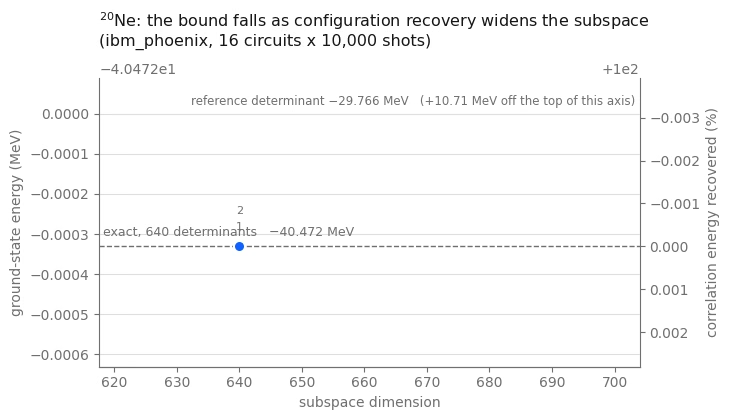
iteration 1: 66 proton x 66 neutron halves -> dimension 640, E = -40.472331 MeV
  iteration 2: 66 proton x 66 neutron halves -> dimension 640, E = -40.472331 MeV

reference determinant    -29.765549 MeV
pooled SQD upper bound          -40.472331 MeV   (subspace dimension 640 of 640)
exact diagonalization    -40.472331 MeV

correlation energy recovered: 100.0%

ประเมินผลลัพธ์

ใช้การตรวจสอบต่อไปนี้เพื่อประเมินผลลัพธ์ของคุณบน backend ระดับ Heron ด้วยการตั้งค่าเหล่านี้

• อัตราการรอดของช็อต (shot survival) บนจำนวนนิวคลีออนทั้งสองวัดสัดส่วนของช็อตที่มีจำนวนโปรตอนและนิวตรอนถูกต้อง ค่านี้อาจลดลงเมื่อ register มีขนาดใหญ่ขึ้น อัตราการรอดที่ใกล้ศูนย์อาจบ่งชี้ปัญหาการรันวงจร (circuit) ให้ตรวจสอบความลึกของ ISA ในขั้นตอนที่ 2 และการปรับเทียบ (calibration) ของ backend ไม่ใช่การประมวลผลภายหลัง

• ลูปการกู้คืน (recovery loop) ควรแสดงมิติของซับสเปซที่คงที่หรือเพิ่มขึ้น และพลังงานที่คงที่หรือลดลงในแต่ละรอบ หากรอบที่ 1 ไปถึง MAX_DIMENSION แล้ว ตัวแก้ปัญหาแบบคลาสสิก (classical solver) มากกว่าการสุ่มตัวอย่างคือข้อจำกัดหลัก

• เศษส่วนที่กู้คืนได้ สำหรับ $^{20}\mathrm{Ne}$ ควรมีค่าสูง เพราะเพดานของ ansatz ที่คำนวณในขั้นตอนที่ 1 คือพื้นที่ดีเทอร์มิแนนต์ 640 ตัวเต็มรูปแบบ การรันนี้จึงเป็นกรณีที่การสุ่มตัวอย่าง ไม่ใช่ความสามารถในการแสดงออก เป็นอุปสรรคเดียว

• การยืนยัน (assertion) ทั้งสอง ในเซลล์ก่อนหน้าตรวจสอบขอบเขตเชิงแปรผัน ขอบเขตที่เพิ่มขึ้นหมายความว่าซับสเปซหยุดเป็นแบบซ้อนกัน (nested) และขอบเขตที่ต่ำกว่าพลังงานที่แท้จริงหมายความว่ามีบางอย่างผิดพลาดกับแฮมิลโทเนียน ไม่ใช่กับฮาร์ดแวร์

อย่างขัดกับสัญชาตญาณ backend ที่มีสัญญาณรบกวนมากกว่าอาจให้ขอบเขตที่ดีกว่า backend ที่สะอาดเล็กน้อย เพราะข้อผิดพลาดสร้างครึ่งคอนฟิกูเรชันที่ถูกต้องซึ่งวงจรในอุดมคติจะไม่มีวันสุ่มได้ และการขยายซับสเปซเชิงแปรผันไม่สามารถเพิ่มไอเกนค่าต่ำสุดของมันได้ การจำลองที่มีสัญญาณรบกวนสามารถแสดงผลแบบเดียวกันได้ บทช่วยสอนนี้แสดงผลนี้ด้วยตัวอย่างจากฮาร์ดแวร์จริง

# IBM Carbon palette: Blue 60 and Blue 80 for data, Gray 100/70/30 for ink and rules
SURFACE, INK, MUTED, RULE = "#ffffff", "#161616", "#6f6f6f", "#c6c6c6"
SERIES, DEEP, PURPLE = "#0f62fe", "#002d9c", "#6929c4"

def convergence_plot(
    history, e_ref, e_exact, title, colour=SERIES, full_dim=None
):
    """Energy against subspace dimension, scaled to the data rather than to the full window.

    A good run lands within a fraction of a percent of the exact answer, so an axis spanning
    reference-to-exact would squash every point onto one line.  The axis is therefore scaled to
    the data (plus the exact line, when there is one), and the right-hand axis carries the
    fraction of the correlation energy so the absolute and relative readings sit side by side.
    """
    dimensions = [h["dimension"] for h in history]
    energies = [h["energy"] for h in history]

    fig, ax = plt.subplots(figsize=(7.4, 4.3), facecolor=SURFACE)
    ax.set_facecolor(SURFACE)
    ax.plot(
        dimensions,
        energies,
        "-o",
        color=colour,
        linewidth=2,
        markersize=8,
        markeredgecolor=SURFACE,
        markeredgewidth=1.5,
        zorder=3,
    )
    stacked = {}
    for h in history:
        # a converged loop repeats the same point; stack the labels so they do not overprint
        key = (round(h["dimension"]), round(h["energy"], 9))
        offset = 12 + 11 * stacked.get(key, 0)
        stacked[key] = stacked.get(key, 0) + 1
        ax.annotate(
            str(h["iteration"]),
            xy=(h["dimension"], h["energy"]),
            xytext=(0, offset),
            textcoords="offset points",
            ha="center",
            fontsize=8,
            color=MUTED,
        )

    span = (max(dimensions) - min(dimensions)) or max(1, max(dimensions) // 4)
    x_left, x_right = (
        min(dimensions) - 0.14 * span,
        max(dimensions) + 0.40 * span,
    )
    ax.set_xlim(x_left, x_right)

    floor = min(energies) if e_exact is None else min(min(energies), e_exact)
    height = max(max(energies) - floor, 1e-3)
    ax.set_ylim(floor - 0.30 * height, max(energies) + 0.42 * height)

    if e_exact is not None:
        ax.axhline(
            e_exact, color=MUTED, linestyle="--", linewidth=1, zorder=1
        )
        label = "exact" + (f", {full_dim:,} determinants" if full_dim else "")
        ax.annotate(
            f"{label}   {e_exact:.3f} MeV".replace("-", "\u2212"),
            xy=(x_left, e_exact),
            xytext=(3, 5),
            textcoords="offset points",
            ha="left",
            va="bottom",
            color=MUTED,
            fontsize=9,
        )

    # the reference determinant is far off this scale; state it rather than plotting it
    ax.annotate(
        f"reference determinant {e_ref:.3f} MeV".replace("-", "\u2212")
        + f"   ({e_ref - max(energies):+.2f} MeV off the top of this axis)".replace(
            "-", "\u2212"
        ),
        xy=(x_right, max(energies) + 0.42 * height),
        xytext=(-3, -12),
        textcoords="offset points",
        ha="right",
        va="top",
        color=MUTED,
        fontsize=8.5,
    )

    if e_exact is not None and abs(e_exact - e_ref) > 1e-9:
        right = ax.twinx()
        low, high = ax.get_ylim()

        def to_percent(e):
            return 100 * (e - e_ref) / (e_exact - e_ref)

        right.set_ylim(to_percent(low), to_percent(high))
        right.set_ylabel("correlation energy recovered (%)", color=MUTED)
        right.tick_params(colors=MUTED)
        for side in ("top", "left"):
            right.spines[side].set_visible(False)
        right.spines["right"].set_color(MUTED)
        right.spines["bottom"].set_color(MUTED)

    ax.set_xlabel("subspace dimension", color=MUTED)
    ax.set_ylabel("ground-state energy (MeV)", color=MUTED)
    ax.set_title(title, color=INK, fontsize=11.5, loc="left", pad=12)
    ax.grid(axis="y", color=RULE, alpha=0.55)
    ax.tick_params(colors=MUTED)
    for side in ("top", "right"):
        ax.spines[side].set_visible(False)
    for side in ("bottom", "left"):
        ax.spines[side].set_color(MUTED)
    fig.tight_layout()
    return fig

convergence_plot(
    result_sd["history"],
    E_REF_SD,
    E_EXACT_SD,
    f"$^{{20}}$Ne: the bound falls as configuration recovery widens the subspace\n"
    f"({backend.name}, {N_CIRCUITS} circuits x {SHOTS:,} shots)",
    full_dim=len(basis_exact_sd),
)
plt.show()

ตัวอย่างฮาร์ดแวร์ขนาดใหญ่

การขยายขนาดเปลี่ยนแปลงเฉพาะอินพุตเท่านั้น ดังนั้นขั้นตอนต่อไปคือการรวมทั้งสี่ขั้นตอนเข้าเป็นฟังก์ชันเดียว และรันสองครั้ง ทั้งสองครั้งบน register ขนาด 40 คิวบิตใน $pf$ shell เหนือแกน $^{40}\mathrm{Ca}$ ด้วยอันตรกิริยา GXPF1 [3]

การรันทั้งสองครั้งแสดงให้เห็นแง่มุมที่แตกต่างกันของการขยายขนาด

• $^{44}\mathrm{Ti}$ ซึ่งมีโปรตอนวาเลนซ์สองตัวและนิวตรอนวาเลนซ์สองตัว มีเบซิสดีเทอร์มิแนนต์ 4,000 ตัว register มีขนาด 40 คิวบิต แต่ปัญหายังเล็กพอที่จะหาไดแอกอนัลได้อย่างแม่นยำบนแล็ปท็อป ดังนั้นคุณสามารถเปรียบเทียบผลลัพธ์จากฮาร์ดแวร์กับค่าอ้างอิงที่แม่นยำได้หลังจากเพิ่มขนาด register

• $^{48}\mathrm{Cr}$ ซึ่งมีโปรตอนวาเลนซ์สี่ตัวและนิวตรอนวาเลนซ์สี่ตัว มีดีเทอร์มิแนนต์ที่สมมาตรอนุญาต 1,963,461 ตัวใน 40 คิวบิตเดียวกัน ตัวแก้ปัญหาแบบหนาแน่น (dense solver) ของบทช่วยสอนนี้ไม่สามารถหาไดแอกอนัลพื้นที่เต็มนั้นได้ ดังนั้นการรันจึงคืนค่า ขอบเขตบนที่เข้มงวดและดีเทอร์มิแนนต์อ้างอิงที่มันปรับปรุงขึ้นมา

สังเกตปริมาณสองอย่างในการรันทั้งสองครั้ง สัดส่วนของกลุ่ม (pool) ที่พอดีกับงบประมาณเกต (gate budget) ที่คงที่จะหดตัวลงเมื่อ pool ขยายขึ้น และ pack_ensemble รายงานว่ามีการรวมเท่าใด ซับสเปซหยุดถูกจำกัดโดยการสุ่มตัวอย่างและเริ่มถูกจำกัดโดย MAX_DIMENSION ซึ่งคือเมทริกซ์ที่ใหญ่ที่สุดที่ตัวแก้ปัญหาแบบคลาสสิกแบบหนาแน่นในที่นี้สร้างขึ้น ในขนาดนี้ การคำนวณระดับการผลิตจริงจะใช้ตัวแก้ปัญหา selected configuration interaction (selected-CI)

รวมขั้นตอนที่ 1–4

ฟังก์ชันต่อไปนี้เรียกใช้ขั้นตอนเดียวกันกับที่อธิบายไว้ ในลำดับเดียวกัน

def sqd_run(snt_file, n_protons, n_neutrons, name, exact=True):
    """The whole workflow for one nucleus.  Returns a record of every stage."""
    # -------------------------Step 1-------------------------
    ms = read_snt(DATA / snt_file, n_protons, n_neutrons)
    sp = m_scheme_states(ms)
    inter = Interaction(ms, sp)
    if sum(1 for s in sp if s.tz == -1) * 2 != len(sp):
        raise ValueError(
            f"{name}: post-selection needs equal proton and neutron state counts"
        )
    reference = reference_determinant(sp, inter, n_protons, n_neutrons)
    e_ref = matrix_element(inter, reference, reference)

    raw = excitation_pool(sp, reference)
    ranked = rank_pool(
        inter, reference, [op for op in raw if conserves_symmetry(sp, op)]
    )
    print(
        f"{name}: {len(sp)} qubits, {n_protons}p + {n_neutrons}n, A = {ms.mass_number}"
    )
    print(
        f"  2p2h pool {len(raw)} raw -> {len(ranked)} symmetry-allowed; "
        f"reference energy {e_ref:.6f} MeV"
    )

    # -------------------------Step 2-------------------------
    costs = excitation_costs(len(sp), ranked, costing_manager)
    circuits, bins, isa = pack_to_budget(
        len(sp),
        reference,
        ranked,
        costs,
        DEPTH_BUDGET,
        N_CIRCUITS,
        pass_manager,
    )
    packed = sum(len(b) for b in bins)
    worst = max(two_qubit_depth(c) for c in isa)
    worst_count = max(two_qubit_count(c) for c in isa)
    print(
        f"  packed {packed} of {len(ranked)} excitations; worst circuit two-qubit depth "
        f"{worst}, {worst_count} two-qubit gates"
    )

    # -------------------------Step 3-------------------------
    # a unique tag per run, so the jobs are findable later
    bit_arrays = sample(isa, SHOTS, JOB_TAGS + [name])
    matrix, probabilities, shots = pool_samples(bit_arrays, sp)
    survival = float(
        probabilities[
            (matrix[:, len(sp) // 2 :].sum(axis=1) == n_protons)
            & (matrix[:, : len(sp) // 2].sum(axis=1) == n_neutrons)
        ].sum()
    )
    print(
        f"  {shots:,} shots -> {len(matrix):,} distinct bitstrings, "
        f"{survival:.1%} of shots with the right nucleon numbers"
    )
    if survival == 0.0:
        raise RuntimeError(
            f"{name}: no shot carried the right nucleon numbers"
        )

    # -------------------------Step 4-------------------------
    result = recovery_loop(
        inter,
        sp,
        matrix,
        probabilities,
        reference,
        n_protons,
        n_neutrons,
        max_iterations=4,
        max_dimension=MAX_DIMENSION,
        seed=42,
    )
    energy = result["energy"]

    full_dim = count_basis(sp, n_protons, n_neutrons)  # cheap, even when huge
    e_exact = None
    if exact:
        full = full_basis(sp, n_protons, n_neutrons)
        if len(full) != full_dim:
            raise AssertionError(
                f"{name}: counted {full_dim} determinants but enumerated "
                f"{len(full)}"
            )
        e_exact, _ = ground_state(inter, full)

    print(f"  reference {e_ref:11.6f} MeV     pooled SQD {energy:11.6f} MeV")
    if e_exact is not None:
        print(
            f"  exact     {e_exact:11.6f} MeV  (dimension {full_dim})  ->  "
            f"{100 * (energy - e_ref) / (e_exact - e_ref):.1f}% of the correlation energy"
        )
        if energy < e_exact - 1e-7:
            raise AssertionError(
                f"{name}: pooled SQD bound is below the exact energy"
            )
    else:
        print(
            f"  no exact reference: the symmetry-allowed basis is {full_dim:,} determinants"
        )
        print(
            f"  the bound captures {energy - e_ref:.6f} MeV of correlation energy"
        )
    print()

    return dict(
        name=name,
        qubits=len(sp),
        pool=len(ranked),
        packed=packed,
        two_qubit=worst,
        two_qubit_gates=worst_count,
        shots=shots,
        distinct=len(matrix),
        survival=survival,
        dimension=len(result["basis"]),
        full_dim=full_dim,
        e_ref=e_ref,
        e_sqd=energy,
        e_exact=e_exact,
        history=result["history"],
        # the subspace and its eigenvector cannot be reconstructed from the summary --
        # they depend on the sampled shots -- so keep them for the scaling analysis
        interaction=inter,
        states=sp,
        reference=reference,
        ranked=ranked,
        basis=result["basis"],
        vector=result["vector"],
    )

pretty = {"20Ne": "$^{20}$Ne", "44Ti": "$^{44}$Ti", "48Cr": "$^{48}$Cr"}

small_scale = dict(
    name="20Ne",
    qubits=len(sp_sd),
    pool=len(ranked_sd),
    packed=PACKED_SD,
    two_qubit=worst_sd,
    two_qubit_gates=worst_count_sd,
    shots=shots_sd,
    distinct=len(matrix_sd),
    survival=shot_survival_sd,
    dimension=len(result_sd["basis"]),
    full_dim=len(basis_exact_sd),
    e_ref=E_REF_SD,
    e_sqd=E_SQD_SD,
    e_exact=E_EXACT_SD,
    history=result_sd["history"],
    interaction=inter_sd,
    states=sp_sd,
    reference=occ_sd,
    ranked=ranked_sd,
    basis=result_sd["basis"],
    vector=result_sd["vector"],
)

$^{44}\mathrm{Ti}$: workflow เดียวกันบน register ขนาด 40 คิวบิต

$pf$ shell เหนือ $^{40}\mathrm{Ca}$ มีออร์บิทัลสี่ตัวต่อชนิด และสถานะย่อยแม่เหล็ก 20 ตัวต่อออร์บิทัล ดังนั้น register จึงมีขนาด 40 คิวบิต โปรตอนวาเลนซ์สองตัวและนิวตรอนวาเลนซ์สองตัวทำให้เกิด $^{44}\mathrm{Ti}$ ซึ่งมีดีเทอร์มิแนนต์ที่สมมาตรอนุญาต 4,000 ตัว — ประมาณหกเท่าของเบซิส $^{20}\mathrm{Ne}$ โดยใช้ 40 คิวบิตแทนที่จะเป็น 24

นี่คือตัวอย่างที่ใหญ่กว่าในสองตัวอย่างที่โน้ตบุ๊กนี้สามารถแก้ได้อย่างแม่นยำ ดังนั้นคุณสามารถเปรียบเทียบ ผลลัพธ์จากฮาร์ดแวร์กับค่าอ้างอิงที่แม่นยำได้

large_scale_verified = sqd_run("gxpf1.snt", 2, 2, "44Ti", exact=True)

44Ti: 40 qubits, 2p + 2n, A = 44
  2p2h pool 1602 raw -> 174 symmetry-allowed; reference energy -44.309387 MeV
  packed 96 of 174 excitations; worst circuit two-qubit depth 272, 285 two-qubit gates
job dap31a02fm4c73f67dp0: 16 circuits x 10,000 shots on ibm_phoenix
  160,000 shots -> 48,170 distinct bitstrings, 18.6% of shots with the right nucleon numbers
  iteration 1: 187 proton x 189 neutron halves -> dimension 3891, E = -47.849086 MeV
  iteration 2: 190 proton x 190 neutron halves -> dimension 4000, E = -47.876666 MeV
  iteration 3: 190 proton x 190 neutron halves -> dimension 4000, E = -47.876666 MeV
  reference  -44.309387 MeV     pooled SQD  -47.876666 MeV
  exact      -47.876666 MeV  (dimension 4000)  ->  100.0% of the correlation energy

$^{48}\mathrm{Cr}$: เกินขีดความสามารถในการหาไดแอกอนัลอย่างแม่นยำของบทช่วยสอนนี้

การเพิ่มโปรตอนสองตัวและนิวตรอนสองตัวใช้ register ขนาด 40 คิวบิตเดียวกัน (4, 4 สำหรับ $^{48}\mathrm{Cr}$) และเพิ่มขนาดเบซิสขึ้นประมาณ 491 เท่า เป็นดีเทอร์มิแนนต์ที่สมมาตรอนุญาต 1,963,461 ตัว เมทริกซ์ นั้นใหญ่เกินกว่าที่บทช่วยสอนนี้จะสร้างได้มาก ดังนั้น exact=False จึงไม่มีพลังงานอ้างอิงที่แม่นยำ มีเพียงขอบเขตเชิงแปรผันและดีเทอร์มิแนนต์อ้างอิงที่มันปรับปรุงขึ้นมาเท่านั้น

มีสองสิ่งที่เปลี่ยนไปในขนาดนี้ และทั้งสองอย่างปรากฏให้เห็นในผลลัพธ์ที่พิมพ์ออกมา pool ขยายไปถึงหลาย ร้อยการกระตุ้นที่อนุญาต ดังนั้นงบประมาณเกตที่คงที่จึงครอบคลุมเพียงส่วนน้อยของมันแทนที่จะเป็นทั้งหมด นอกจากนี้ ซับสเปซผลคูณที่ตัวอย่างครอบคลุมมีขนาดใหญ่กว่า MAX_DIMENSION ดังนั้นตัวแก้ปัญหาแบบหนาแน่น จึงตัดทอนมันตามน้ำหนักที่สุ่มมา ขอบเขตยังคงเข้มงวดแต่สามารถแม่นยำน้อยกว่าขอบเขตที่คำนวณ จากคอนฟิกูเรชันที่สุ่มมาทั้งหมด การคำนวณระดับการผลิตจริงจะเก็บตัวอย่างไว้ และใช้ตัวแก้ปัญหาที่รองรับซับสเปซที่ใหญ่กว่า

large_scale_unverified = sqd_run("gxpf1.snt", 4, 4, "48Cr", exact=False)

48Cr: 40 qubits, 4p + 4n, A = 48
  2p2h pool 5536 raw -> 582 symmetry-allowed; reference energy -93.041237 MeV
  packed 96 of 582 excitations; worst circuit two-qubit depth 224, 279 two-qubit gates
job dap32a02fm4c73f67eog: 16 circuits x 10,000 shots on ibm_phoenix
  160,000 shots -> 55,436 distinct bitstrings, 18.6% of shots with the right nucleon numbers
  iteration 1: 223 proton x 223 neutron halves -> dimension 3977, E = -96.481598 MeV
  iteration 2: 223 proton x 223 neutron halves -> dimension 3977, E = -96.481598 MeV
  reference  -93.041237 MeV     pooled SQD  -96.481598 MeV
  no exact reference: the symmetry-allowed basis is 1,963,461 determinants
  the bound captures -3.440361 MeV of correlation energy

ประเมินผลลัพธ์โดยไม่มีค่าอ้างอิงที่แม่นยำ

การรัน $^{48}\mathrm{Cr}$ ไม่มีค่าอ้างอิงที่แม่นยำภายในบทช่วยสอนนี้ ใช้ตัวอย่างที่มีอยู่ เพื่อประเมินการลู่เข้า (convergence) และเปรียบเทียบกับพื้นฐานการเลือกแบบคลาสสิก โดยไม่ต้องใช้เวลา QPU เพิ่มเติมหรือหาไดแอกอนัลพื้นที่เต็ม

มันลู่เข้าแล้วหรือยัง เรียงลำดับดีเทอร์มิแนนต์ที่เก็บไว้ใหม่ตามน้ำหนักในไอเกนเวกเตอร์ที่ลู่เข้าแล้ว และซับสเปซจะกลายเป็นแบบซ้อนกัน (nested) ดังนั้นการหาไดแอกอนัลของบล็อก $d \times d$ ที่นำหน้าสำหรับลำดับของ $d$ จะติดตามการลดลงของขอบเขตข้ามขนาดซับสเปซสองทศวรรษ หากมันยังลดลงอย่างรวดเร็วที่ $d$ ที่ใหญ่ที่สุด ขีดจำกัดมิติของตัวแก้ปัญหาแบบคลาสสิกคือข้อจำกัดหลักและ MAX_DIMENSION คือ พารามิเตอร์ที่ควรเพิ่ม หากมันคงตัวแล้ว การเพิ่มดีเทอร์มิแนนต์ที่เก็บไว้เพิ่มเติมจะให้การปรับปรุงเพียงเล็กน้อย ความคืบหน้าเพิ่มเติมอาจต้องอาศัยการสุ่มตัวอย่างคอนฟิกูเรชันเพิ่มเติม แฮมิลโทเนียน ถูกสร้างเพียงครั้งเดียวที่ขนาดเต็ม และทุกขั้นเป็นบล็อกหลักของมัน ดังนั้นการกวาดทั้งหมด จึงมีต้นทุนเท่ากับการสร้างเมทริกซ์หนึ่งครั้งแทนที่จะเป็นหนึ่งครั้งต่อขั้น

การสุ่มตัวอย่างควอนตัมเปรียบเทียบกับการเลือกแบบคลาสสิกอย่างไร เปรียบเทียบกับซับสเปซที่มีขนาด เท่ากันซึ่งเลือกโดยขั้นตอนการเลือกแบบคลาสสิก โดยนำ pool ที่จัดอันดับด้วยทฤษฎีการรบกวน (perturbation theory) ตามลำดับคะแนน ขยายซับสเปซผลคูณให้มีมิติเท่ากัน แล้วหาไดแอกอนัลแทน ทั้งสองเส้นโค้งเป็น ขอบเขตบนที่เข้มงวดบนแฮมิลโทเนียนเดียวกัน ดังนั้นเส้นใดที่อยู่ต่ำกว่าที่มิติเท่ากันจึงเลือกดีเทอร์มิแนนต์ ที่ดีกว่า การเปรียบเทียบนี้ตัดสินว่าการสุ่มตัวอย่างด้วยฮาร์ดแวร์ช่วยปรับปรุงค่าประมาณพลังงาน เมื่อเทียบกับพื้นฐานแบบคลาสสิกนี้หรือไม่

ซับสเปซนี้ไม่ได้ถูกเลือกสำหรับสถานะกระตุ้น การกู้คืนคอนฟิกูเรชันนำทางซับสเปซ โดยใช้การครอบครองของสถานะพื้น ดังนั้นไอเกนค่าที่สูงกว่าจึงห่างจากการลู่เข้ามากกว่าค่าต่ำสุดมาก และพลังงานการกระตุ้นแรกออกมาสูงกว่าค่า $2^+$ ที่วัดได้มาก การไปถึงสถานะกระตุ้น อย่างถูกต้องต้องใช้ซับสเปซที่ถูกเลือกมาสำหรับสถานะเหล่านั้น

def subspace_scaling(
    inter, basis, vector, points=18, smallest=32, largest=None
):
    """Nested Rayleigh-Ritz sweep: the lowest eigenvalue of the leading d x d block, for a ladder of d.

    Reordering the basis by descending weight in the converged eigenvector makes every subspace in
    the ladder a subset of the next, so the energies fall monotonically and each one is a valid
    variational bound.  H is built once at full size; each rung is a principal block.
    """
    order = np.argsort(-(np.abs(vector) ** 2))
    ordered = [basis[i] for i in order]
    weights = (np.abs(vector) ** 2)[order]
    if (
        largest is not None
    ):  # cap the ladder so two subspaces end at a common dimension
        ordered, weights = ordered[:largest], weights[:largest]
    H = subspace_hamiltonian(inter, ordered)
    dimensions = np.unique(
        np.geomspace(smallest, len(ordered), points).astype(int)
    )
    rows = [
        (
            int(d),
            float(
                eigh(H[:d, :d], eigvals_only=True, subset_by_index=[0, 0])[0]
            ),
        )
        for d in dimensions
    ]
    return rows, np.cumsum(weights)

def classical_selection(
    inter, sp, reference, ranked, target, n_protons, n_neutrons
):
    """The subspace classical perturbative ranking would pick, grown to `target` dimension.

    Same product construction as the sampled subspace, and the same truncation discipline -- half
    configurations are offered to `grow_subspace` in order of importance and it takes as many as
    fit.  The only difference from the sampled path is where the ordering comes from: PT2 score
    here, measured sampling weight there.  So the comparison isolates *which determinants got
    chosen* and nothing else.

    Truncating by any other rule would not be a fair baseline.  Slicing an arbitrarily ordered
    list, for instance, keeps determinants by accident rather than by importance and makes the
    classical subspace look worse than classical selection really is.
    """
    p_ref = tuple(i for i in reference if sp[i].tz == -1)
    n_ref = tuple(i for i in reference if sp[i].tz == +1)
    reached = {reference}
    proton_order, neutron_order = [p_ref], [n_ref]
    seen_p, seen_n = {p_ref}, {n_ref}
    product_budget = 4 * target

    for op, _, _ in ranked:  # ranked is already in descending PT2 score
        h1, h2, v1, v2 = op
        fresh = {
            tuple(sorted(set(d) - {h1, h2} | {v1, v2}))
            for d in reached
            if {h1, h2} <= set(d) and not {v1, v2} & set(d)
        }
        reached |= fresh
        for det in fresh:  # first appearance fixes a half's rank
            half_p = tuple(i for i in det if sp[i].tz == -1)
            half_n = tuple(i for i in det if sp[i].tz == +1)
            if half_p not in seen_p:
                seen_p.add(half_p)
                proton_order.append(half_p)
            if half_n not in seen_n:
                seen_n.add(half_n)
                neutron_order.append(half_n)
        if len(proton_order) * len(neutron_order) > product_budget:
            # Half-configuration products over-count the subspace, because only the
            # symmetry-allowed ones survive `product_subspace`.  Stopping on the product
            # count alone can therefore leave the basis far short of `target`, so check
            # the dimension actually realized and widen the budget if it falls short.
            trial, _, _ = grow_subspace(
                sp,
                [p_ref],
                [n_ref],
                proton_order,
                neutron_order,
                n_protons,
                n_neutrons,
                max_dimension=target,
            )
            if len(trial) >= target:
                break
            product_budget *= 2

    basis, _, _ = grow_subspace(
        sp,
        [p_ref],
        [n_ref],
        proton_order,
        neutron_order,
        n_protons,
        n_neutrons,
        max_dimension=target,
    )
    return basis

run = large_scale_unverified
if "basis" not in run:
    raise RuntimeError(
        "this cell needs the subspace and eigenvector that sqd_run now returns; "
        "re-run the sqd_run definition and the 48Cr cell"
    )

print(
    f"{run['name']}: sweeping nested subspaces of the sampled basis "
    f"(dimension {run['dimension']})"
)
sampled_rows, cumulative = subspace_scaling(
    run["interaction"], run["basis"], run["vector"]
)

print(
    f"{run['name']}: building the classically selected subspace at the same dimension"
)
classical_basis = classical_selection(
    run["interaction"],
    run["states"],
    run["reference"],
    run["ranked"],
    run["dimension"],
    4,
    4,
)
# Both subspaces must be scored at the same dimension.  Symmetry filtering can still leave
# the classical construction short of the target when the ranked pool runs out, so take the
# dimension both actually reach, cap both ladders there, and verify they agree.
common_dim = min(sampled_rows[-1][0], len(classical_basis))
if common_dim < sampled_rows[-1][0]:
    sampled_rows, _ = subspace_scaling(
        run["interaction"], run["basis"], run["vector"], largest=common_dim
    )
classical_rows, _ = subspace_scaling(
    run["interaction"],
    classical_basis,
    ground_state(run["interaction"], classical_basis)[1],
    largest=common_dim,
)
if sampled_rows[-1][0] != classical_rows[-1][0]:
    raise RuntimeError(
        f"comparison dimensions differ: sampled {sampled_rows[-1][0]}, "
        f"classical {classical_rows[-1][0]}"
    )

advantage = sampled_rows[-1][1] - classical_rows[-1][1]
direction = "lower" if advantage < 0 else "higher"
verdict = "beats" if advantage < 0 else "does not beat"
descent = next(
    e for d, e in reversed(sampled_rows) if d <= sampled_rows[-1][0] / 2
)
for fraction in (0.90, 0.99):
    count = int(np.searchsorted(cumulative, fraction) + 1)
    print(
        f"  {fraction:.0%} of the eigenvector norm sits on {count} determinants "
        f"({count / run['full_dim']:.1e} of the {run['full_dim']:,}-determinant space)"
    )
print(
    f"  bound still falling {1000 * (sampled_rows[-1][1] - descent):+.1f} keV "
    f"over the last doubling of dimension"
)
print(
    f"  sampled {sampled_rows[-1][1]:.6f} MeV vs classically selected "
    f"{classical_rows[-1][1]:.6f} MeV at a verified common dimension of "
    f"{classical_rows[-1][0]:,}"
)
print(
    f"  -> the sampled subspace is {abs(advantage) * 1000:.0f} keV {direction}"
)

48Cr: sweeping nested subspaces of the sampled basis (dimension 3977)
48Cr: building the classically selected subspace at the same dimension
  90% of the eigenvector norm sits on 107 determinants (5.4e-05 of the 1,963,461-determinant space)
  99% of the eigenvector norm sits on 593 determinants (3.0e-04 of the 1,963,461-determinant space)
  bound still falling -15.6 keV over the last doubling of dimension
  sampled -96.481598 MeV vs classically selected -95.314510 MeV at a verified common dimension of 3,957
  -> the sampled subspace is 1167 keV lower

fig, axes = plt.subplots(1, 2, figsize=(11.2, 4.0), facecolor=SURFACE)

# left: two nested convergence curves on the same axes
ax = axes[0]
ax.set_facecolor(SURFACE)
ax.plot(
    [d for d, _ in sampled_rows],
    [e for _, e in sampled_rows],
    "-o",
    color=SERIES,
    linewidth=2,
    markersize=5,
    markeredgecolor=SURFACE,
    markeredgewidth=1,
    zorder=4,
    label="sampled on the QPU",
)
ax.plot(
    [d for d, _ in classical_rows],
    [e for _, e in classical_rows],
    "--s",
    color=MUTED,
    linewidth=1.6,
    markersize=4,
    markeredgecolor=SURFACE,
    markeredgewidth=1,
    zorder=3,
    label="classically selected, same size",
)
ax.axhline(run["e_ref"], color=RULE, linestyle=":", linewidth=1.2, zorder=1)
ax.annotate(
    f"reference determinant {run['e_ref']:.2f} MeV".replace("-", "\u2212"),
    xy=(sampled_rows[-1][0], run["e_ref"]),
    xytext=(-2, 4),
    textcoords="offset points",
    ha="right",
    va="bottom",
    color=MUTED,
    fontsize=8,
)

# mark the gap between the two curves at the largest dimension, not either curve alone
edge = sampled_rows[-1][0]
ax.plot(
    [edge, edge],
    [classical_rows[-1][1], sampled_rows[-1][1]],
    "-",
    color=SERIES,
    linewidth=1.0,
    alpha=0.7,
    zorder=2,
)
ax.annotate(
    f"{abs(advantage) * 1000:.0f} keV {direction}\nat equal dimension",
    xy=(edge, 0.5 * (classical_rows[-1][1] + sampled_rows[-1][1])),
    xytext=(-8, 0),
    textcoords="offset points",
    ha="right",
    va="center",
    color=SERIES,
    fontsize=8.5,
)

ax.set_xscale("log")
ax.set_xlim(sampled_rows[0][0] * 0.75, edge * 1.5)
ax.set_xlabel("subspace dimension", color=MUTED)
ax.set_ylabel("variational upper bound (MeV)", color=MUTED)
ax.set_title(
    f"{pretty[run['name']]}: the bound, and the subspace it {verdict}",
    color=INK,
    fontsize=11,
    loc="left",
    pad=10,
)
legend = ax.legend(frameon=False, fontsize=8.5, loc="lower left")
for text in legend.get_texts():
    text.set_color(MUTED)

# right: why a few thousand determinants can bound two million
ax = axes[1]
ax.set_facecolor(SURFACE)
ranks = np.arange(1, len(cumulative) + 1)
ax.plot(ranks, 100 * cumulative, "-", color=DEEP, linewidth=2, zorder=3)
for fraction, style, label_y in ((0.90, ":", 46), (0.99, "--", 24)):
    count = int(np.searchsorted(cumulative, fraction) + 1)
    ax.axvline(count, color=MUTED, linestyle=style, linewidth=1, zorder=1)
    ax.annotate(
        f"{fraction:.0%} of the norm\non {count} determinants",
        xy=(count, label_y),
        xytext=(7, 0),
        textcoords="offset points",
        ha="left",
        va="center",
        color=MUTED,
        fontsize=8.5,
    )
ax.set_xscale("log")
ax.set_xlim(0.8, len(cumulative) * 2.6)
ax.set_ylim(0, 104)
ax.set_xlabel("determinants, ordered by weight", color=MUTED)
ax.set_ylabel("cumulative share of the eigenvector (%)", color=MUTED)
ax.set_title(
    f"Sparsity: {run['full_dim']:,} determinants in the sector",
    color=INK,
    fontsize=11,
    loc="left",
    pad=10,
)

for ax in axes:
    ax.grid(axis="y", color=RULE, alpha=0.55)
    ax.tick_params(colors=MUTED, labelsize=8.5)
    for side in ("top", "right"):
        ax.spines[side].set_visible(False)
    for side in ("bottom", "left"):
        ax.spines[side].set_color(MUTED)
fig.tight_layout()
plt.show()

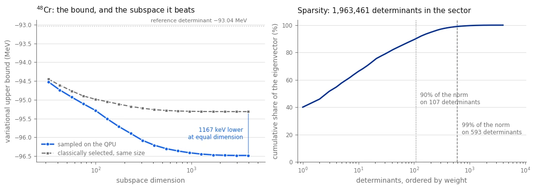
เปรียบเทียบการรันทั้งสามครั้ง

พลังงานสัมบูรณ์ไม่สามารถเปรียบเทียบข้ามนิวเคลียสและอันตรกิริยาที่แตกต่างกันได้ ดังนั้นให้เน้นที่สัดส่วนของพลังงานสหสัมพันธ์ (correlation energy) ที่กู้คืนได้ข้ามการรันต่างๆ ในกรณีที่มีค่าอ้างอิงที่แม่นยำ นอกจากนี้ให้เปรียบเทียบความลึกของวงจรและสัดส่วน ของช็อตที่ถูกทิ้ง

runs = [small_scale, large_scale_verified, large_scale_unverified]

print(
    f"{'run':>6}  {'qubits':>6}  {'pool':>9}  {'2q depth':>8}  {'2q gates':>8}  "
    f"{'shots kept':>10}  {'dim':>6}  {'of':>9}  {'% corr':>7}"
)
for r in runs:
    fraction = (
        "--"
        if r["e_exact"] is None
        else f"{100 * (r['e_sqd'] - r['e_ref']) / (r['e_exact'] - r['e_ref']):.1f}%"
    )
    coverage = "{}/{}".format(r["packed"], r["pool"])
    print(
        f"{r['name']:>6}  {r['qubits']:>6}  {coverage:>9}  "
        f"{r['two_qubit']:>8}  {r['two_qubit_gates']:>8}  {r['survival']:>9.1%}  "
        f"{r['dimension']:>6}  {(r['full_dim'] or 0):>9,}  {fraction:>7}"
    )

print()
for r in runs:
    exact = (
        f"exact {r['e_exact']:11.6f}"
        if r["e_exact"] is not None
        else "exact  unavailable"
    )
    print(
        f"{r['name']:>6}   reference {r['e_ref']:11.6f}   pooled SQD {r['e_sqd']:11.6f}   {exact} MeV"
    )

run  qubits       pool  2q depth  2q gates  shots kept     dim         of   % corr
  20Ne      24      78/78       228       234      31.5%     640        640   100.0%
  44Ti      40     96/174       272       285      18.6%    4000      4,000   100.0%
  48Cr      40     96/582       224       279      18.6%    3977  1,963,461       --

  20Ne   reference  -29.765549   pooled SQD  -40.472331   exact  -40.472331 MeV
  44Ti   reference  -44.309387   pooled SQD  -47.876666   exact  -47.876666 MeV
  48Cr   reference  -93.041237   pooled SQD  -96.481598   exact  unavailable MeV

# Left: how much of the correlation energy was recovered, where the exact answer is known.
# Right: the bound itself for the run that has nothing to score against.
scored = [r for r in runs if r["e_exact"] is not None]

fig, ax = plt.subplots(figsize=(6.4, 3.9), facecolor=SURFACE)
ax.set_facecolor(SURFACE)
labels = [
    f"{pretty[r['name']]}\n{r['qubits']} qubits\n{r['full_dim']:,} determinants"
    for r in scored
]
fractions = [
    100 * (r["e_sqd"] - r["e_ref"]) / (r["e_exact"] - r["e_ref"])
    for r in scored
]
shades = [SERIES, DEEP, PURPLE]
bars = ax.bar(
    labels, fractions, width=0.46, color=shades[: len(scored)], zorder=3
)
for bar, fraction, r in zip(bars, fractions, scored):
    ax.annotate(
        f"{fraction:.1f}%",
        xy=(bar.get_x() + bar.get_width() / 2, fraction),
        xytext=(0, 5),
        textcoords="offset points",
        ha="center",
        va="bottom",
        color=INK,
        fontsize=10,
    )
    ax.annotate(
        f"dim {r['dimension']:,}",
        xy=(bar.get_x() + bar.get_width() / 2, 3),
        ha="center",
        va="bottom",
        color=SURFACE,
        fontsize=8.5,
    )
ax.axhline(100, color=MUTED, linestyle="--", linewidth=1, zorder=1)
ax.annotate(
    "exact diagonalization",
    xy=(-0.45, 100),
    xytext=(0, 4),
    textcoords="offset points",
    ha="left",
    va="bottom",
    color=MUTED,
    fontsize=8.5,
)
ax.set_ylim(0, 118)
ax.set_ylabel("correlation energy recovered (%)", color=MUTED)
ax.set_title(
    f"Where the exact answer is known ({backend.name})",
    color=INK,
    fontsize=11,
    loc="left",
    pad=10,
)
ax.grid(axis="y", color=RULE, alpha=0.55)
ax.tick_params(colors=MUTED, labelsize=8.5)
for side in ("top", "right"):
    ax.spines[side].set_visible(False)
for side in ("bottom", "left"):
    ax.spines[side].set_color(MUTED)
fig.tight_layout()
plt.show()

# the same convergence view as the walkthrough, for the run with no exact reference
convergence_plot(
    large_scale_unverified["history"],
    large_scale_unverified["e_ref"],
    None,
    f"{pretty[large_scale_unverified['name']]}: "
    f"{large_scale_unverified['full_dim']:,} determinants, no exact answer to score against\n"
    f"({backend.name}, {N_CIRCUITS} circuits x {SHOTS:,} shots)",
    colour=DEEP,
)
plt.show()

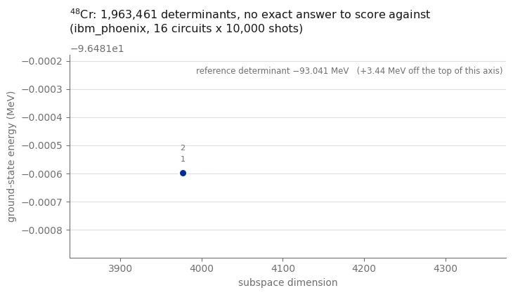
สรุป

workflow เดียว ไม่เปลี่ยนแปลงยกเว้นอินพุตของมัน รันบน QPU ที่ขนาดปัญหาสามแบบ ได้แก่ ปัญหา 24 คิวบิต ที่คุณสามารถตรวจสอบได้อย่างแม่นยำ ปัญหา 40 คิวบิตที่คุณยังสามารถตรวจสอบได้อย่างแม่นยำ และปัญหา 40 คิวบิต ที่มีสถานะเบซิสเกือบสองล้านสถานะ ซึ่งเกินขีดความสามารถในการหาไดแอกอนัลอย่างแม่นยำของบทช่วยสอนนี้

การรันทั้งสามครั้งแสดงให้เห็นประเด็นต่อไปนี้

• ขั้นตอนควอนตัมมีหน้าที่เพียงเสนอดีเทอร์มิแนนต์เท่านั้น วงจรถูกกำหนดตายตัว มาจากทฤษฎีการรบกวน อันดับสอง และไม่เคยถูกปรับให้เหมาะสม ไม่มีสิ่งใดใน workflow ที่ต้องการให้แอมพลิจูดของมัน แม่นยำ ต้องการเพียงให้ support ของมันมีประโยชน์เท่านั้น การหาไดแอกอนัลแบบคลาสสิกในซับสเปซที่เลือกให้ ขอบเขตบนเชิงแปรผัน แม้ว่าขอบเขตจะแปรผันไปตามคอนฟิกูเรชันที่สุ่มมา

• การกระตุ้นคิวบิต (qubit excitations) ลดความลึกของวงจร เนื่องจากมีเพียง support เท่านั้นที่สำคัญ บล็อกการกระตุ้นแบบเฟอร์มิออน จึงสามารถแทนที่ด้วยการกระตุ้นคิวบิตได้ ซึ่งต้นทุนของมันไม่เพิ่มขึ้นตามระยะห่างระหว่าง ออร์บิทัลที่มันเชื่อมต่อ ขั้นตอนที่ 2 วัดการประหยัดนี้บน backend จริง ซึ่งเป็นความแตกต่าง ระหว่างวงจรที่พอดีอยู่ในขอบเขตความสอดคล้อง (coherence) และวงจรที่ไม่พอดี

• การกู้คืนคอนฟิกูเรชันนำตัวอย่างที่มีสัญญาณรบกวนกลับมาใช้ใหม่ ทุกช็อตที่มีจำนวนโปรตอนหรือนิวตรอนไม่ถูกต้องจะถูกซ่อมแซม เทียบกับค่าประมาณการครอบครองปัจจุบัน แทนที่จะถูกทิ้ง และครึ่งคอนฟิกูเรชันที่ซ่อมแซมแล้วแต่ละอัน สามารถเพิ่มคอนฟิกูเรชันเข้าไปในซับสเปซได้ การขยายซับสเปซเชิงแปรผันไม่สามารถเพิ่มไอเกนค่า ต่ำสุดของมันได้ บทช่วยสอนนี้แสดงการกู้คืนคอนฟิกูเรชันโดยใช้ตัวอย่างจากฮาร์ดแวร์

• ข้อจำกัดหลักเปลี่ยนไปเมื่อคุณขยายขนาด ที่ 24 คิวบิต ansatz สามารถไปถึงคำตอบที่แม่นยำได้ และมีเพียงการสุ่มตัวอย่างเท่านั้นที่ขวางทาง ที่ 40 คิวบิตด้วยนิวคลีออนวาเลนซ์สี่ตัวต่อชนิด งบประมาณเกต ครอบคลุมเพียงส่วนน้อยของ pool และตัวแก้ปัญหาแบบคลาสสิกแบบหนาแน่นจำกัดซับสเปซ การรู้ว่า อันไหนในสามอย่างนี้กำลังจำกัดคุณอยู่คือทักษะเชิงปฏิบัติที่ workflow นี้สอน

ขั้นตอนถัดไป

คำแนะนำ

สำรวจแหล่งข้อมูลที่เกี่ยวข้องต่อไปนี้

• การหาไดแอกอนัลควอนตัมแบบอิงตัวอย่างของแฮมิลโทเนียนเคมี: อัลกอริทึมเดียวกันที่ประยุกต์ใช้กับโครงสร้างอิเล็กทรอนิกส์ โดยใช้ตัวแก้ปัญหา selected-CI ของ SQD addon

• เอกสาร SQD addon: ยูทิลิตี้สำหรับ post-selection, การสุ่มตัวอย่างย่อย (subsampling) และการกู้คืนคอนฟิกูเรชัน

• อัลกอริทึมการหาไดแอกอนัลควอนตัม: คอร์สเต็มเกี่ยวกับการหาไดแอกอนัลซับสเปซ รวมถึงตัวแปร Krylov

• บทนำสู่การแปล (transpilation): ตัวเลือกของ pass manager ที่สำคัญเมื่อวงจรถูกครอบงำด้วยเกตสองคิวบิต

• โหมดการรัน (execution modes): สำรวจโหมด batch สำหรับการจัดตารางงานที่เป็นอิสระต่อกัน

ส่วนขยายที่ควรพิจารณา

• แทนที่ตัวแก้ปัญหาแบบหนาแน่น (dense solver) MAX_DIMENSION คือเพดานของทุกอย่างที่ขนาด $^{48}\mathrm{Cr}$ และ np.linalg.eigh บนเมทริกซ์หนาแน่นคือสาเหตุ การสร้างแฮมิลโทเนียนที่ถูกฉายภาพ (projected) เดียวกันเป็นเมทริกซ์แบบ sparse และใช้ตัวหาไอเกน (eigensolver) แบบวนซ้ำ เช่น scipy.sparse.linalg.eigsh หรือตัวแก้ปัญหาแบบ Davidson หรือ selected-CI ที่ออกแบบสำหรับ อันตรกิริยานิวเคลียร์แบบสองวัตถุ อาจรองรับซับสเปซที่ใหญ่กว่าได้ ขีดจำกัดในทางปฏิบัติขึ้นอยู่กับความ sparse ของเมทริกซ์ หน่วยความจำที่มีอยู่ และการลู่เข้าของตัวแก้ปัญหา และบทช่วยสอนนี้ไม่ได้ทำการเปรียบเทียบประสิทธิภาพของส่วนขยายนั้น qiskit_addon_sqd.fermion.solve_sci ของ SQD addon ไม่ใช่ตัวทดแทนที่ใช้แทนกันได้ทันที เพราะมันห่อหุ้ม ตัวแก้ปัญหาโครงสร้างอิเล็กทรอนิกส์และต้องการอินทิกรัลแบบหนึ่งวัตถุและสองวัตถุในรูปแบบนั้น ดังนั้นโครงสร้างผลคูณของโปรตอน $\times$ นิวตรอนที่ใช้ร่วมกันจึงไม่เพียงพอในตัวมันเอง การใช้มันหมายถึงการแมป อันตรกิริยาแบบ shell model ของสมการ (1) ไปเป็นอินทิกรัลเหล่านั้น และตรวจสอบผลลัพธ์เทียบกับ พลังงานที่แม่นยำที่โน้ตบุ๊กนี้คำนวณไว้แล้ว

• เพิ่มการทำ batching และ subsampling workflow SQD แบบ pooled ที่เผยแพร่จะหาไดแอกอนัลตัวอย่างย่อยที่เป็นอิสระหลายชุด ต่อรอบและเก็บชุดที่ดีที่สุดไว้ บทช่วยสอนนี้ใช้ batch เดียวต่อรอบ ซึ่งไม่เป็นอันตรายต่อ ขอบเขตเชิงแปรผัน แต่ไม่ให้ข้อมูลความแปรปรวนที่บ่งชี้ว่าช็อตเพิ่มเติมจะช่วยได้หรือไม่

• สถานะกระตุ้นและเซกเตอร์อื่นๆ ไอเกนค่าที่สูงกว่าของแฮมิลโทเนียนของแต่ละซับสเปซเป็นขอบเขตบน ของสถานะกระตุ้นในเซกเตอร์สมมาตรเดียวกัน และการรันที่ $M_J \neq 0$ จะไปถึงเซกเตอร์อื่นๆ การตรวจสอบ $2^+$ ในขั้นตอนที่ 1 เป็นครึ่งหนึ่งของการคำนวณนี้อยู่แล้ว

• พื้นที่แบบจำลองข้ามเชลล์ (cross-shell) ภาวะคู่ (parity) เป็นไปตามข้อกำหนดโดยอัตโนมัติภายในเชลล์หลักเดียว ซึ่ง เป็นเหตุผลที่มันไม่มีบทบาทใดๆ ที่นี่ พื้นที่ $sd$-$pf$ ผสมภาวะคู่ของ $\ell$ เข้าด้วยกัน ทำให้ภาวะคู่เป็น ข้อจำกัดที่สี่อย่างแท้จริง ซึ่งทั้งการซ่อมแซมแบบ Hamming-weight ของ SQD และการสร้างผลคูณ จะตรวจจับไม่ได้ด้วยตัวมันเอง

• นิวเคลียสมวลคี่ (odd-mass) reference_determinant ต้องการจำนวนวาเลนซ์เป็นเลขคู่ในแต่ละชนิด เพราะการเติมแบบจับคู่ที่ผกผันเวลา (time-reversed) คือสิ่งที่บังคับให้ $M_J = 0$ นิวเคลียสคี่ต้องการ เป้าหมาย $M_J$ เป็นเลขครึ่งจำนวนเต็มและค่าอ้างอิงที่ไม่จับคู่

ภาคผนวก

ส่วนนี้อธิบายเหตุผลเบื้องหลังตัวช่วยที่แนะนำในส่วน การตั้งค่า

เหตุใดการปรับสเกลตามการพึ่งพามวลจึงไม่ใช่ตัวเลือก

อันตรกิริยาแบบ shell model เชิงประจักษ์ถูกฟิตที่มวลหนึ่งและนำไปใช้ข้ามสายไอโซโทป โดย สมาชิกเมทริกซ์แบบสองวัตถุถูกปรับสเกลเป็น $(A/A_{\mathrm{ref}})^{p}$ ไฟล์อันตรกิริยาทั้งสองมี $p = -0.3$ โดย $A_{\mathrm{ref}} = 18$ สำหรับตระกูล USD และ $42$ สำหรับ GXPF1 บนบรรทัดหัว แบบสองวัตถุของไฟล์ .snt ตัวเลขทั้งสองนั้นอยู่ในตำแหน่งที่ความถี่ออสซิลเลเตอร์และพลังงานแกนกลางน่าจะอยู่ ซึ่งทำให้อ่านผิดได้ง่าย การอ่านเลขชี้กำลังเป็นพลังงานแกนกลางคงที่จะเพิ่มค่าชดเชยปลอมให้กับ ทุกสมาชิกแนวทแยงมุม และ ทำให้การปรับสเกลหายไป ซึ่งเปลี่ยนพลังงานสหสัมพันธ์ไป สองสามเปอร์เซ็นต์ การตรวจสอบสมมาตรในขั้นตอนที่ 1 เพียงอย่างเดียวไม่สามารถยืนยันสเกลพลังงานได้ การเปรียบเทียบพลังงานการกระตุ้น $2^+$ ที่วัดเป็น MeV กับการทดลองให้การตรวจสอบเพิ่มเติมต่อ การปรับสเกลตามมวล พลังงานการกระตุ้นคือความต่างระหว่างระดับพลังงาน ดังนั้นมันจึงไม่ ตรวจจับค่าชดเชยคงที่ที่ถูกใส่เข้าไปในพลังงานทั้งหมด

เหตุใดค่าอ้างอิงจึงถูกหาด้วยการค้นหา ไม่ใช่การเติม

ค่าอ้างอิงที่ชัดเจนที่สุดคือดีเทอร์มิแนนต์ที่เติมพลังงานอนุภาคเดี่ยวต่ำสุด มันไม่ใช่ ดีเทอร์มิแนนต์ที่มีพลังงานต่ำสุด เพราะแนวทแยงมุมของสมการ (1) มีพจน์สองวัตถุ $\sum_{i<j} \langle ij \| ij \rangle$ และอันตรกิริยาแบบจับคู่ (pairing) ชอบการครอบครองคู่ $(+m_j, -m_j)$ ที่ผกผันเวลาใน $|m_j|$ ที่ใหญ่ที่สุดที่มีอยู่อย่างมาก ใน $sd$ shell นั่นคือ ความต่างระหว่างคู่ $m_j = \pm 1/2$ กับคู่ $m_j = \pm 5/2$ ของ $0d_{5/2}$ และมีค่าประมาณ 1 MeV ใน $pf$ shell มีค่าใกล้เคียง 2 มากกว่า เนื่องจากพลังงานอ้างอิงกำหนดจุดศูนย์ของตัวชี้วัด "พลังงานสหสัมพันธ์ที่กู้คืนได้" การเลือกที่ไม่ดีจะทำให้ตัวชี้วัดนั้นพองตัวและให้จุดเริ่มต้น ที่แม่นยำน้อยกว่า

การจำกัดให้เป็นการเติมแบบจับคู่ทำให้การค้นหาแบบละเอียดถี่ถ้วนมีต้นทุนต่ำ โดยมีผู้สมัคร $\binom{n_{\mathrm{pairs}}}{k}$ ต่อชนิด (มากที่สุดไม่กี่พัน) และรับประกัน $M_J = 0$ ในทุกกรณีในบทช่วยสอนนี้ ที่สามารถตรวจสอบเทียบกับการแจกแจงแบบเต็มได้ การค้นหาจะคืนค่าดีเทอร์มิแนนต์ที่มีแนวทแยงมุม ต่ำสุดทั่วโลก ซึ่งเป็นองค์ประกอบเดี่ยวที่ใหญ่ที่สุดของสถานะพื้นที่แท้จริงด้วย

เหตุใดจึงใช้แอมพลิจูดอันดับหนึ่ง ไม่ใช่มุมสองระดับที่แม่นยำ

การหาไดแอกอนัลแฮมิลโทเนียน $2 \times 2$ ในพื้นที่ $\{|\Phi_{\mathrm{ref}}\rangle, |\alpha\rangle\}$ ให้มุมการผสม $\theta_{\mathrm{exact}} = \tfrac{1}{2}\arctan(2V/\Delta)$ อาจดูน่าดึงดูดที่จะเรียกมันว่าตัวเลือก ที่ถูกต้องสำหรับคู่ระดับที่แยกอิสระ ใน ansatz นี้ บล็อกการกระตุ้นหลายสิบบล็อกทำงาน ต่อเนื่องกันบนค่าอ้างอิงเดียวกัน ดังนั้นการปรับให้เหมาะสมแต่ละบล็อกแยกกันจึงไม่จำเป็นต้อง ปรับวงจรที่ประกอบขึ้นให้เหมาะสมด้วย

บทบาทของวงจรเป็นตัวกำหนดการเลือกมุม เนื่องจาก $|\tfrac{1}{2}\arctan(2x)| \le |x|$ สำหรับทุกจำนวนจริง $x$ มุมที่แม่นยำจึงมีขนาดเล็กกว่าเสมอ เมื่อเทียบกับแอมพลิจูดอันดับหนึ่ง $t = V/\Delta$ และดังนั้นจึงเหลือแอมพลิจูดมากกว่าเสมอ บนดีเทอร์มิแนนต์อ้างอิง วงจรที่เก็บแอมพลิจูดไว้บนค่าอ้างอิงมากกว่าจะคืนค่า ค่าอ้างอิงบ่อยกว่าและดีเทอร์มิแนนต์กระตุ้นที่แตกต่างกันน้อยกว่า สำหรับ pooled SQD ผลลัพธ์ที่มีประโยชน์ของช็อต คือดีเทอร์มิแนนต์ที่ขั้นตอนแบบคลาสสิกยังไม่เคยเห็นมาก่อน ซึ่งเป็นแรงจูงใจให้ใช้มุมที่ใหญ่กว่าในบทช่วยสอนนี้ ทั้งสองมุมไม่จำเป็นต้องแม่นยำ เพราะการหาไดแอกอนัลแบบคลาสสิกทิ้งแอมพลิจูดของวงจร ไปทั้งหมดและหาแอมพลิจูดของตัวเองใหม่

เหตุใด pooled SQD จึงสามารถใช้การกระตุ้นคิวบิตได้

การกระตุ้นแบบเฟอร์มิออน $T = a_{v_1}^\dagger a_{v_2}^\dagger a_{h_2} a_{h_1}$ แมปภายใต้ Jordan-Wigner ไปเป็น Pauli string แปดตัว โดยแต่ละตัวมีตัวดำเนินการ $Z$ บนทุกคิวบิตระหว่างดัชนี ที่อยู่นอกสุด string เหล่านี้เข้ารหัสเครื่องหมายของเฟอร์มิออน และต้นทุนของมันเพิ่มขึ้นตามช่วง ซึ่งสำหรับการกระตุ้นแบบโปรตอน-นิวตรอนคือ register ทั้งหมด

การลบสิ่งเหล่านั้นออกจะได้ตัวดำเนินการการกระตุ้นคิวบิตของ Yordanov และคณะ [5] มันเป็นตัวดำเนินการ ที่ต่างออกไป สถานะที่มันเตรียมแตกต่างจากสถานะแบบเฟอร์มิออนตรงที่เครื่องหมายของ แอมพลิจูดของมัน และการแจกแจงการสุ่มตัวอย่างทั้งสองแบบอาจแตกต่างกันอย่างมาก สิ่งที่มันไม่เปลี่ยนแปลง คือดีเทอร์มิแนนต์ใดมีแอมพลิจูดไม่เป็นศูนย์ เพราะแต่ละบล็อกยังคงหมุนภายในพื้นที่สองมิติเดียวกัน $\{|d\rangle, |d'\rangle\}$ สำหรับทุกดีเทอร์มิแนนต์ $d$ ที่มันกระทำอยู่ และมันยังคง อนุรักษ์จำนวนนิวคลีออนทั้งสอง $M_J$ และภาวะคู่ไว้อย่างแม่นยำ ดังนั้นชุดดีเทอร์มิแนนต์ที่เข้าถึงได้ จึงเหมือนกัน และชุดที่เข้าถึงได้คือสิ่งเดียวที่ pooled SQD ใช้ การหา ไดแอกอนัลแบบคลาสสิกกำหนดแอมพลิจูดของตัวเองไม่ว่ากรณีใด ขั้นตอนที่ 2 ตรวจสอบข้อกล่าวอ้างเรื่อง support ที่เหมือนกันบน ตัวดำเนินการจริงจาก pool และวัดสิ่งที่การแทนที่นี้ประหยัดได้

ข้อจำกัดคือน้ำหนักของการสุ่มตัวอย่างแตกต่างกัน ดังนั้นทั้งสองโครงสร้างจะไม่ค้นพบ ดีเทอร์มิแนนต์ในลำดับเดียวกันที่จำนวนช็อตจำกัด เนื่องจากการจัดอันดับที่ตัดสินว่าการกระตุ้นใด จะเข้าไปในวงจรเป็นแบบคลาสสิกและไม่เปลี่ยนแปลง และขั้นตอนแบบคลาสสิกจะกำหนดน้ำหนักใหม่ให้ทุกอย่างอยู่ดี ความแตกต่างในน้ำหนักการสุ่มตัวอย่างจึงเป็นการแลกเปลี่ยนเพื่อลดความลึกของวงจร

เหตุใด $M_J$ จึงเป็นของขั้นตอนผลคูณ

การเลือกภายหลัง (post-selection) และการกู้คืนคอนฟิกูเรชันต่างก็ทำงานบนน้ำหนักแฮมมิง (Hamming weight) จำนวนโปรตอนในครึ่งหนึ่งของ register และจำนวนนิวตรอนในอีกครึ่งหนึ่ง $M_J = M_p + M_n$ ไม่ได้อยู่ในรูปแบบนั้น มันเป็นคุณสมบัติของคอนฟิกูเรชันโปรตอนที่จับคู่กับคอนฟิกูเรชันนิวตรอน ช็อตที่ครึ่งโปรตอนและครึ่งนิวตรอนแต่ละส่วนมีจำนวนนิวคลีออนถูกต้องมีครึ่งคอนฟิกูเรชันที่ใช้ได้สองส่วนแม้ เมื่อค่า $M_J$ ของพวกมันไม่หักล้างกัน เพราะครึ่งโปรตอนที่ $M_p = +1$ ใช้ได้ดีอย่างสมบูรณ์เมื่อ จับคู่กับครึ่งนิวตรอนที่ $M_n = -1$ การกรองทั้งช็อตด้วย $M_J$ รวมจะทิ้งทั้งสองครึ่ง ไป ในขณะที่การกำหนด $M_J$ บนผลคูณที่รวมกลับมาใหม่จะเก็บพวกมันไว้ เหตุผลเดียวกันนี้อธิบายว่าทำไม recover_configurations จึงไม่จำเป็นต้องมีแนวคิดเรื่อง $M_J$ เพื่อให้มีประโยชน์ในกรณีนี้

เอกสารอ้างอิง

1. J. Robledo-Moreno, M. Motta, H. Haas, et al., "Chemistry beyond the scale of exact diagonalization on a quantum-centric supercomputer", Science Advances 11, eadu9991 (2025). arXiv:2405.05068

2. B. A. Brown and W. A. Richter, "New USD Hamiltonians for the sd shell", Physical Review C 74, 034315 (2006). The embedded usda.snt file carries the USDA parameters as tabulated by W. A. Richter, S. Mkhize and B. A. Brown, "sd-shell observables for the USDA and USDB Hamiltonians", Physical Review C 78, 064302 (2008).

3. M. Honma, T. Otsuka, B. A. Brown and T. Mizusaki, "Effective interaction for pf-shell nuclei", Physical Review C 65, 061301(R) (2002).

4. B. Huron, J. P. Malrieu and P. Rancurel, "Iterative perturbation calculations of ground and excited state energies from multiconfigurational zeroth-order wavefunctions", The Journal of Chemical Physics 58, 5745 (1973).

5. Y. S. Yordanov, D. R. M. Arvidsson-Shukur and C. H. W. Barnes, "Efficient quantum circuits for quantum computational chemistry", Physical Review A 102, 062612 (2020).

6. National Nuclear Data Center, Evaluated Nuclear Structure Data File, Brookhaven National Laboratory. แหล่งที่มาของพลังงานการกระตุ้น $2^+$ ที่วัดได้ซึ่งอ้างถึงในขั้นตอนที่ 1