การเพิ่มประสิทธิภาพหลายวัตถุประสงค์แบบประมาณเชิงควอนตัม

ประมาณการการใช้งาน: 10 นาทีบนโปรเซสเซอร์ Heron r2 (หมายเหตุ: เป็นเพียงการประมาณการเท่านั้น เวลารันจริงของคุณอาจแตกต่างออกไป)

ผลลัพธ์การเรียนรู้

บทเรียนนี้แก้ปัญหาการเพิ่มประสิทธิภาพพอร์ตโฟลิโอที่จำกัดจำนวนสินทรัพย์: เมื่อกำหนดให้ถือสินทรัพย์เพียง $K$ รายการพอดี ให้สมดุลระหว่างวัตถุประสงค์ด้านความเสี่ยง ผลตอบแทน และการกระจายความเสี่ยง เพื่อหาเซตของพอร์ตโฟลิโอที่เหมาะสมที่สุด

เมื่อทำบทเรียนนี้เสร็จ คุณจะเข้าใจ:

• วิธีแสดงปัญหาการเลือกพอร์ตโฟลิโอที่มีสามวัตถุประสงค์ขัดแย้งกัน — ความเสี่ยงต่ำ ผลตอบแทนสูง และการกระจายความเสี่ยงที่ดี — เป็นปัญหาการเพิ่มประสิทธิภาพเชิงควอนตัม

• วิธีที่ circuit QAOA เพียงตัวเดียว เมื่อกวาดผ่านชุดน้ำหนักของวัตถุประสงค์ จะลาก แนวหน้า Pareto ของพอร์ตโฟลิโอที่แลกเปลี่ยนได้อย่างเหมาะสมที่สุดออกมา

• วิธีที่ XY mixer ทำให้การค้นหาอยู่ภายใน subspace "เลือกสินทรัพย์ K รายการพอดี" จึงไม่ต้องใช้พจน์ลงโทษ และความเป็นไปได้ถูกบังคับด้วยการ post-select bitstring ที่วัดได้

• วิธีฝึกมุมของ circuit ด้วยซิมูเลเตอร์แบบ matrix-product-state ในขนาดที่ใหญ่เกินกว่าจะเพิ่มประสิทธิภาพแบบแม่นตรงได้ ตาม Kotil et al. (arXiv:2503.22797)

สิ่งที่ควรรู้ก่อน

แนะนำให้คุณคุ้นเคยกับ:

• เวิร์กโฟลว์ Qiskit patterns (map, optimize, execute, post-process)

• พื้นฐานของ QAOA

ภูมิหลัง

ผู้จัดการพอร์ตโฟลิโอแทบไม่เคยเพิ่มประสิทธิภาพตัวเลขเพียงตัวเดียว พวกเขาต้องการให้ผลตอบแทนสูง ความเสี่ยง (ความแปรปรวนของผลตอบแทนเหล่านั้น) ต่ำ และการถือครองกระจายไปตามภาคส่วนต่างๆ เพื่อไม่ให้พอร์ตโฟลิโอเสี่ยงต่อส่วนใดส่วนหนึ่งของตลาดมากเกินไป เป้าหมายเหล่านี้ขัดแย้งกัน: สินทรัพย์ที่ให้ผลตอบแทนสูงที่สุดมักผันผวนที่สุด และการกระจุกตัวในภาคส่วนที่ร้อนแรงเพียงภาคเดียวส่งผลเสียต่อการกระจายความเสี่ยง

ไม่มีพอร์ตโฟลิโอที่ "ดีที่สุด" เพียงหนึ่งเดียว แต่มี แนวหน้า Pareto คือเซตของพอร์ตโฟลิโอที่คุณไม่สามารถปรับปรุงวัตถุประสงค์หนึ่งได้โดยไม่เสียอีกวัตถุประสงค์หนึ่ง เป้าหมายของเราคือวาดแผนที่แนวหน้านั้นเพื่อให้ผู้ตัดสินใจเลือกการแลกเปลี่ยนที่ตนต้องการได้

เรากำหนดปัญหาเป็นการเลือกสินทรัพย์ $K$ รายการจาก $N$ รายการพอดี (สินทรัพย์แต่ละรายการอยู่ในหรือนอกพอร์ตโฟลิโอ — หนึ่ง qubit ต่อหนึ่งสินทรัพย์) Hamiltonian สามตัวเข้ารหัสวัตถุประสงค์ทั้งสาม เรารวมมันด้วยน้ำหนัก $c$ ที่อยู่บน simplex (ผลรวมเป็นหนึ่ง) และ QAOA sampler คืนพอร์ตโฟลิโอที่ดีสำหรับน้ำหนักแต่ละชุดที่เลือก การกวาดน้ำหนักคือการกวาดความสำคัญสัมพัทธ์ของความเสี่ยงเทียบกับผลตอบแทนเทียบกับการกระจายความเสี่ยง และยูเนียนของพอร์ตโฟลิโอที่สุ่มตัวอย่างทั้งหมดจะลากแนวหน้า Pareto ออกมา

ก่อนอื่นเราเดินผ่านเวิร์กโฟลว์ทั้งหมดบนตัวอย่างเล็กๆ แปดสินทรัพย์ที่เราตรวจสอบได้ด้วยการไล่ทุกกรณี แล้วจึงรันวิธีเดียวกันนี้บนอินสแตนซ์ 40 สินทรัพย์ที่มีขนาดเหมาะกับฮาร์ดแวร์ควอนตัม

บทเรียนนี้สอนเวิร์กโฟลว์ (การแมป การฝึกมุม การสุ่มตัวอย่างแบบมีข้อจำกัด และการประมวลผลภายหลังแบบ Pareto) ไม่ได้แสดงให้เห็น quantum advantage ที่ขนาด 40 สินทรัพย์ที่ใช้ในที่นี้ การสุ่มตัวอย่างแบบสุ่มสม่ำเสมอทำงานได้ดีพอๆ กับ QAOA sampler และเราแสดงการเปรียบเทียบนั้นอย่างชัดเจน

ข้อกำหนด

ก่อนเริ่มบทเรียนนี้ ตรวจสอบให้แน่ใจว่าคุณติดตั้งสิ่งต่อไปนี้แล้ว:

• Qiskit SDK v2.0 ขึ้นไป พร้อมการรองรับ visualization

• Qiskit Runtime v0.22 ขึ้นไป (pip install qiskit-ibm-runtime)

• Qiskit Aer (pip install qiskit-aer)

• addon ของ Qiskit ชื่อ Optimization mapper (pip install qiskit-addon-opt-mapper) และ QAOA training pipeline ที่ตรึงไว้ที่แท็ก v0.1.0: pip install "git+https://github.com/qiskit-community/qaoa_training_pipeline.git@v0.1.0"

• moocore สำหรับการคำนวณแนวหน้า Pareto และ hypervolume (pip install moocore)

การตั้งค่า

นำเข้าไลบรารีที่ใช้ตลอดบทเรียนและกำหนด random seed เพื่อให้ทำซ้ำได้

# Added by doQumentation — installs the packages this notebook needs if they are missing
import importlib.util

_needed = {"matplotlib": "matplotlib", "moocore": "moocore", "numpy": "numpy", "qaoa_training_pipeline": "qaoa-training-pipeline", "qiskit": "qiskit", "qiskit_addon_opt_mapper": "qiskit-addon-opt-mapper", "qiskit_aer": "qiskit-aer", "qiskit_ibm_runtime": "qiskit-ibm-runtime", "scipy": "scipy"}
_missing = [pip for module, pip in _needed.items()
            if importlib.util.find_spec(module) is None]
# One at a time, so a package that fails to install does not block the others
for _pip in _missing:
    %pip install -q {_pip}
if not _missing:
    print("\u2713 All required packages are installed")

import numpy as np
import matplotlib.pyplot as plt
from math import comb
from moocore import hypervolume, filter_dominated, is_nondominated

from qiskit import QuantumCircuit
from qiskit.circuit import ParameterVector
from qiskit.circuit.library import qaoa_ansatz
from qiskit.quantum_info import SparsePauliOp
from qiskit.transpiler import generate_preset_pass_manager
from qiskit_aer.primitives import SamplerV2 as AerSampler
from qiskit_addon_opt_mapper.problems import OptimizationProblem
from qaoa_training_pipeline.training import ScipyTrainer
from qaoa_training_pipeline.evaluation import (
    StatevectorEvaluator,
    MPSAerEvaluator,
)

np.random.seed(42)
sampler = AerSampler(seed=42)  # local simulator for the small-scale example
print("Setup complete.")

Setup complete.

ตัวอย่างซิมูเลเตอร์ขนาดเล็ก

เราเริ่มด้วยสินทรัพย์แปดรายการจากหกภาคส่วน และเลือกสินทรัพย์ $K=4$ รายการพอดี เมื่อมีสินทรัพย์เพียงแปดรายการ จะมีพอร์ตโฟลิโอที่ถูกต้องเพียง $\binom{8}{4}=70$ พอร์ต เราจึงตรวจสอบผลลัพธ์เชิงควอนตัมกับการค้นหาแบบครบถ้วนได้ภายหลัง

ขั้นตอนที่ 1: แมปอินพุตคลาสสิกไปเป็นปัญหาควอนตัม

สินทรัพย์แต่ละรายการคือหนึ่ง qubit; bitstring อย่าง 10110010 คือพอร์ตโฟลิโอ (เลข 1 คือสินทรัพย์ที่เราถือ) เราต้องการสามองค์ประกอบ: ข้อมูลตลาด Hamiltonian ของวัตถุประสงค์ทั้งสาม และ circuit ที่เสนอเฉพาะพอร์ตโฟลิโอที่มีสินทรัพย์ $K$ รายการพอดีเท่านั้น

# --- Small-scale universe: 8 assets across 6 sectors ---
tickers = ["AAPL", "XOM", "JPM", "JNJ", "KO", "AMT", "AMZN", "SLB"]
sectors = [
    "Tech",
    "Energy",
    "Finance",
    "Health",
    "Staples",
    "REIT",
    "Tech",
    "Energy",
]
n_assets = len(tickers)
K = 4  # choose exactly K assets
n_obj = 3  # risk, return, diversification

# Annualized expected returns
mu = np.array([0.28, 0.12, 0.22, 0.05, 0.08, 0.10, 0.32, 0.15])

# Annualized covariance matrix (the "risk" model)
sigma = np.array(
    [
        [0.070, 0.010, 0.020, 0.008, 0.005, 0.012, 0.045, 0.011],
        [0.010, 0.065, 0.015, 0.006, 0.004, 0.008, 0.009, 0.050],
        [0.020, 0.015, 0.055, 0.010, 0.007, 0.015, 0.018, 0.014],
        [0.008, 0.006, 0.010, 0.030, 0.012, 0.009, 0.007, 0.005],
        [0.005, 0.004, 0.007, 0.012, 0.025, 0.006, 0.004, 0.003],
        [0.012, 0.008, 0.015, 0.009, 0.006, 0.045, 0.011, 0.007],
        [0.045, 0.009, 0.018, 0.007, 0.004, 0.011, 0.085, 0.010],
        [0.011, 0.050, 0.014, 0.005, 0.003, 0.007, 0.010, 0.072],
    ]
)

# Diversification score: number of cross-sector pairs in the portfolio.
# D[i,j] = 0.5 when assets i and j are in different sectors, so x^T D x counts
# the cross-sector pairs. More cross-sector pairs = better diversified.
D = np.array(
    [
        [1.0 if sectors[i] != sectors[j] else 0.0 for j in range(n_assets)]
        for i in range(n_assets)
    ]
)
np.fill_diagonal(D, 0.0)
D = D / 2

print(f"{n_assets} assets, choose K={K}, {n_obj} objectives")
for t, s, m in zip(tickers, sectors, mu):
    print(f"  {t:5s} ({s:8s})  expected return {m:5.0%}")

8 assets, choose K=4, 3 objectives
  AAPL  (Tech    )  expected return   28%
  XOM   (Energy  )  expected return   12%
  JPM   (Finance )  expected return   22%
  JNJ   (Health  )  expected return    5%
  KO    (Staples )  expected return    8%
  AMT   (REIT    )  expected return   10%
  AMZN  (Tech    )  expected return   32%
  SLB   (Energy  )  expected return   15%

# Each objective becomes a Hamiltonian whose lowest-energy bitstrings are the
# best portfolios for that objective. The opt-mapper turns a plain
# min/max problem over binary variables into the equivalent Ising operator.
def build_risk_hamiltonian(sigma, n):
    """Minimize portfolio variance x^T sigma x  (quadratic -> ZZ terms)."""
    prob = OptimizationProblem("risk")
    prob.binary_var_list(n)
    prob.minimize(quadratic=sigma)
    op, _ = prob.to_ising()
    return op.simplify()

def build_return_hamiltonian(mu, n):
    """Maximize expected return mu . x  (linear -> Z terms)."""
    prob = OptimizationProblem("return")
    prob.binary_var_list(n)
    prob.maximize(linear=mu)
    op, _ = prob.to_ising()
    return op.simplify()

def build_diversity_hamiltonian(D, n):
    """Maximize cross-sector pairs x^T D x  (quadratic -> ZZ terms)."""
    prob = OptimizationProblem("diversity")
    prob.binary_var_list(n)
    prob.maximize(quadratic=D)
    op, _ = prob.to_ising()
    return op.simplify()

H_risk = build_risk_hamiltonian(sigma, n_assets)
H_return = build_return_hamiltonian(mu, n_assets)
H_diversity = build_diversity_hamiltonian(D, n_assets)
cost_ops = [H_risk, H_return, H_diversity]

for name, op in zip(["risk", "return", "diversity"], cost_ops):
    print(f"H_{name:10s}: {op.size} Pauli terms")

H_risk      : 36 Pauli terms
H_return    : 8 Pauli terms
H_diversity : 34 Pauli terms

การบังคับ "สินทรัพย์ K รายการพอดี" โดยไม่ใช้พจน์ลงโทษ เทคนิคที่พบบ่อยคือเพิ่มพจน์ลงโทษที่ลงโทษพอร์ตโฟลิโอที่มีขนาดไม่ถูกต้อง แต่วิธีนี้เชื่อมทุก qubit เข้ากับ qubit อื่นทุกตัว ทำให้ circuit ลึกขึ้นมากหลัง transpile แต่เราใช้ XY mixer ซึ่งเคลื่อนสถานะ QAOA ระหว่าง bitstring ที่มี Hamming weight เท่ากันเท่านั้น หากเริ่มจากสถานะที่เลือกสินทรัพย์ $K$ รายการไว้แล้ว ทุกพอร์ตโฟลิโอที่ circuit สำรวจก็จะมีสินทรัพย์ $K$ รายการพอดีเช่นกัน ข้อจำกัดถูกสร้างไว้ในโครงสร้างของ circuit แทนที่จะบังคับด้วยพจน์ลงโทษ

เราเตรียมสถานะเริ่มต้นอย่างประหยัด: หมุนแต่ละ qubit ให้ "เปิด" ด้วยความน่าจะเป็น $K/N$ เมื่อจำกัดเฉพาะผลลัพธ์ที่มีสินทรัพย์ $K$ รายการ จะได้สถานะน้ำหนักเท่ากันในอุดมคติ (Dicke) เราจึงเก็บเฉพาะ bitstring ที่วัดได้ซึ่งมีเลข 1 พอดี $K$ ตัว — ขั้นตอนที่เรียกว่า post-selection

def xy_mixer(n):
    """Line XY mixer: couples neighboring qubits with XX+YY. Conserves the number
    of selected assets (Hamming weight), so cardinality is preserved automatically.
    Using a line (not a full ring) keeps the circuit shallow and hardware-friendly."""
    terms = [
        (pauli, [i, i + 1], 1) for i in range(n - 1) for pauli in ("XX", "YY")
    ]
    return SparsePauliOp.from_sparse_list(terms, n)

def product_init(n, k):
    """Cheap initial state: each qubit rotated so P(selected) = k/n. Zero two-qubit
    gates. Post-selecting its weight-k outcomes reproduces the ideal Dicke state."""
    qc = QuantumCircuit(n)
    theta = 2 * np.arcsin(np.sqrt(k / n))
    for q in range(n):
        qc.ry(theta, q)
    return qc

# Combine the three objectives with weights c (bound later, at sampling time).
p_layers = 1
c = ParameterVector("c", n_obj)
# Negate the objective so the sampling phase separator matches the sign the angles
# were trained under (the trainer maximizes the negated sum); binding below keeps +gamma.
combined_cost_op = sum(
    -c[k] * H_k for k, H_k in enumerate(cost_ops)
).simplify()

ansatz = qaoa_ansatz(
    combined_cost_op,
    reps=p_layers,
    initial_state=product_init(n_assets, K),
    mixer_operator=xy_mixer(n_assets),
)
ansatz.measure_all()

betas = [p for p in ansatz.parameters if p.name.startswith("β")]
gammas = [p for p in ansatz.parameters if p.name.startswith("γ")]
print(f"Qubits: {ansatz.num_qubits} | QAOA layers: {p_layers}")
print(
    f"Tunable angles: {len(betas)} beta + {len(gammas)} gamma, plus {n_obj} objective weights"
)

Qubits: 8 | QAOA layers: 1
Tunable angles: 1 beta + 1 gamma, plus 3 objective weights

ขั้นตอนที่ 2: ปรับแต่งปัญหาสำหรับการรันบนฮาร์ดแวร์ควอนตัม

ก่อนรัน circuit นามธรรมจะถูก transpile เป็น gate แบบเนทีฟของฮาร์ดแวร์ ในขนาดเล็กนี้เราเพียงตรวจสอบต้นทุน: circuit ลึกเท่าใด และใช้ gate สอง qubit กี่ตัว? (gate สอง qubit เป็นแหล่งสัญญาณรบกวนหลักบนอุปกรณ์จริง)

# Bind dummy angle values so we can transpile and measure the circuit's size.
dummy = {p: 0.1 for p in ansatz.parameters}
test_pm = generate_preset_pass_manager(optimization_level=1)
test_qc = test_pm.run(ansatz.assign_parameters(dummy))

print(f"Circuit depth          : {test_qc.depth()}")
print(
    f"Two-qubit gate depth   : {test_qc.depth(lambda x: len(x.qubits) > 1)}"
)
print(f"Two-qubit gate count   : {test_qc.num_nonlocal_gates()}")

Circuit depth          : 25
Two-qubit gate depth   : 23
Two-qubit gate count   : 42

ขั้นตอนที่ 3: รันโดยใช้ Qiskit primitives

สองระยะ ก่อนอื่นเรา ฝึก มุม QAOA หนึ่งครั้ง โดยใช้น้ำหนักวัตถุประสงค์เท่ากัน ด้วยซิมูเลเตอร์ statevector แบบแม่นตรง เพื่อหาค่า $\beta,\gamma$ ที่ดี จากนั้นเรา กวาด เวกเตอร์น้ำหนักจำนวนมากทั่ว simplex และสุ่มตัวอย่าง circuit ที่แต่ละจุดเพื่อรวบรวมพอร์ตโฟลิโอตัวเลือก เนื่องจากระหว่างการกวาดมีเพียงน้ำหนักวัตถุประสงค์ที่เปลี่ยน (ไม่ใช่มุมที่ฝึกแล้ว) เวกเตอร์น้ำหนักทั้งหมดจึงถูกส่งในงานแบบ batch เพียงงานเดียว

# Train the angles with equal objective weights.
# The trainer maximizes energy, so we negate the (to-be-minimized) objective sum.
training_op = sum(-1.0 / n_obj * H_k for H_k in cost_ops).simplify()

# Linear-ramp initialization (Sack and Serbyn, arXiv:2101.05742)
dt = 0.75
grid = np.arange(1, p_layers + 1) - 0.5
init_params = np.concatenate((1 - grid * dt / p_layers, grid * dt / p_layers))

trainer = ScipyTrainer(
    StatevectorEvaluator(), minimize_args={"options": {"maxiter": 300}}
)
print("Training QAOA angles (exact statevector)...")
result_train = trainer.train(
    cost_op=training_op,
    mixer=xy_mixer(n_assets),
    initial_state=product_init(n_assets, K),
    params0=init_params,
)
opt = result_train["optimized_params"]
opt_betas, opt_gammas = opt[:p_layers], opt[p_layers:]
print(f"Trained beta : {opt_betas}")
print(f"Trained gamma: {opt_gammas}")

Training QAOA angles (exact statevector)...
Trained beta : [3.329186967386619]
Trained gamma: [3.4449804324291033]

def random_uniform_simplex(n_samples, n_obj=3):
    """n_samples weight vectors spread uniformly over the (n_obj-1)-simplex."""
    s = np.zeros((n_samples, n_obj + 1))
    s[:, 1:-1] = np.random.rand(n_samples, n_obj - 1)
    s[:, -1] = 1
    s = np.sort(s, axis=1)
    return np.diff(s, axis=1)

# Bind the trained angles, leaving the objective weights c free for the sweep.
param_map = {betas[i]: opt_betas[i] for i in range(p_layers)}
param_map.update({gammas[i]: opt_gammas[i] for i in range(p_layers)})
ansatz_bound = ansatz.assign_parameters(param_map)

n_samples, shots = 200, 500
c_vecs = random_uniform_simplex(n_samples, n_obj)

print(f"Sampling {n_samples} weight vectors x {shots} shots...")
result = sampler.run([(ansatz_bound, c_vecs)], shots=shots).result()

# Collect every distinct bitstring seen across all weight vectors.
all_bitstrings = set()
for s in range(n_samples):
    for bs in result[0].data.meas.get_counts(s):
        # get_counts is little-endian; reverse so bit i = asset i
        all_bitstrings.add(bs.replace(" ", "")[::-1])
print(f"Distinct portfolios sampled: {len(all_bitstrings)}")

Sampling 200 weight vectors x 500 shots...
Distinct portfolios sampled: 256

ขั้นตอนที่ 4: ประมวลผลภายหลังและคืนผลลัพธ์ในรูปแบบคลาสสิกที่ต้องการ

เราเก็บเฉพาะพอร์ตโฟลิโอที่เป็นไปได้ (สินทรัพย์ $K$ รายการพอดีจากขั้นตอน post-selection) ให้คะแนนแต่ละพอร์ตบนวัตถุประสงค์ทั้งสาม และสกัด แนวหน้า Pareto: พอร์ตโฟลิโอที่ไม่ถูกเอาชนะในทุกวัตถุประสงค์พร้อมกัน Hypervolume เป็นตัวเลขเดียวที่สรุปว่าแนวหน้าครอบงำปริภูมิวัตถุประสงค์ได้มากเพียงใด และยิ่งมากยิ่งดี

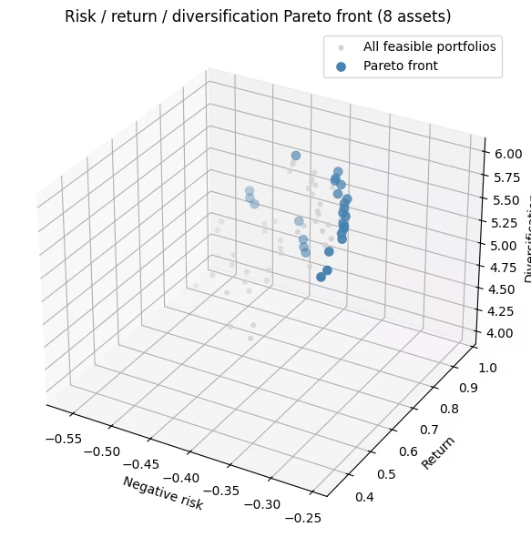
ด้วย 100,000 shot บน bitstring เพียง 256 แบบ การรันนี้เห็นครบทั้ง 70 พอร์ตโฟลิโอที่ถูกต้อง ดังนั้นที่ขนาดนี้จึงเป็นการตรวจสอบแบบไล่ทุกกรณีว่า pipeline เชื่อมต่อถูกต้อง ไม่ใช่หลักฐานว่า QAOA พบแนวหน้า

def evaluate_portfolio(bitstring, sigma, mu, D):
    """Score one portfolio on all three objectives (all framed as 'bigger is better')."""
    x = np.array([int(b) for b in bitstring])
    # negative risk, return, diversification (cross-sector pairs)
    return np.array([-(x @ sigma @ x), x @ mu, x @ D @ x])

# Post-select feasible portfolios, then score them.
feasible = [bs for bs in all_bitstrings if bs.count("1") == K]
fis = np.array([evaluate_portfolio(bs, sigma, mu, D) for bs in feasible])

pareto_front = filter_dominated(fis, maximise=True)
ref_point = fis.min(axis=0)
qmoo_hv = hypervolume(fis, ref=ref_point, maximise=True)

print(
    f"Feasible portfolios found : {len(feasible)} of {comb(n_assets, K)} possible"
)
print(f"Pareto-front portfolios   : {len(pareto_front)}")
print(f"Hypervolume               : {qmoo_hv:.4f}")

Feasible portfolios found : 70 of 70 possible
Pareto-front portfolios   : 26
Hypervolume               : 0.2487

fig = plt.figure(figsize=(8, 6))
ax = fig.add_subplot(111, projection="3d")
ax.scatter(
    fis[:, 0],
    fis[:, 1],
    fis[:, 2],
    c="lightgray",
    s=12,
    label="All feasible portfolios",
)
ax.scatter(
    pareto_front[:, 0],
    pareto_front[:, 1],
    pareto_front[:, 2],
    c="steelblue",
    s=45,
    label="Pareto front",
)
ax.set_xlabel("Negative risk")
ax.set_ylabel("Return")
ax.set_zlabel("Diversification")
ax.set_title("Risk / return / diversification Pareto front (8 assets)")
ax.legend()
plt.tight_layout()
plt.show()

ตัวอย่างฮาร์ดแวร์ขนาดใหญ่

ตอนนี้เวิร์กโฟลว์เดียวกันบน 40 สินทรัพย์ (8 ภาคส่วน × 5) โดยเลือก $K=6$ สี่สิบ qubit ใหญ่เกินกว่าจะจำลองแบบแม่นตรง (statevector ที่มีแอมพลิจูด $2^{40}$ ตัว) จึงไม่สามารถเพิ่มประสิทธิภาพมุมแบบที่ทำกับแปดสินทรัพย์ได้ และ circuit แบบหนาแน่นจะลึกเกินไปสำหรับฮาร์ดแวร์ปัจจุบัน พอร์ตโฟลิโอที่ถูกต้อง $\binom{40}{6} \approx 3.8$M พอร์ตยังน้อยพอที่จะแจงนับด้วยวิธีคลาสสิก ซึ่งเราใช้ตอนท้ายเป็นเกณฑ์มาตรฐานแบบแม่นตรง มีหลายอย่างที่เปลี่ยนไป และ วิธีการไม่มีอะไรเปลี่ยนอีก:

1. ฝึกมุมด้วยซิมูเลเตอร์ matrix-product-state (MPS) ไม่ใช่ statevector แบบแม่นตรง ตามเอกสารอ้างอิง (Kotil et al.) เรากำหนดน้ำหนักวัตถุประสงค์ให้เท่ากัน เพิ่มประสิทธิภาพ β, γ ชุดเดียวบนซิมูเลเตอร์ MPS และนำกลับมาใช้กับทุกเวกเตอร์น้ำหนักในการกวาด (เราฝึกที่ขนาดที่เรารันจริง — ไม่มีการถ่ายโอนมุมจากเล็กไปใหญ่)

2. ทำให้โมเดลความเสี่ยงเบาบางเพื่อให้พอดีกับฮาร์ดแวร์ ความแปรปรวนร่วมเต็มรูปแบบเชื่อมสินทรัพย์ทั้ง 780 คู่ เราเก็บเฉพาะการเชื่อมที่แข็งแรงที่สุดและเดินสายถูกที่สุดด้วย การตัดทอน QAP ที่คำนึงถึงความสำคัญ และเชื่อมแต่ละภาคส่วนเป็นวงแหวนเบาๆ สำหรับพจน์ความหลากหลาย วิธีนี้ทำให้วัตถุประสงค์ยังมีความหมาย ขณะที่ทำให้ circuit มีขนาดเป็นมิตรกับฮาร์ดแวร์

3. ทำให้ circuit ตื้นและให้คะแนนอย่างซื่อตรง การเดินสายเป็นแบบสุ่ม เราจึง transpile ด้วยหลาย seed และเก็บอันที่ตื้นที่สุด (และไม่ต้องใช้เวลาควอนตัม) พอร์ตโฟลิโอจะถูก ให้คะแนนเทียบกับวัตถุประสงค์เต็มรูปแบบที่แท้จริง เสมอ การทำให้เบาบางมีผลต่อรูปร่างของ circuit เท่านั้น ไม่ใช่วิธีตัดสินพอร์ตโฟลิโอ

ทำไมต้องตัดทอน QAP?

การเก็บการเชื่อมที่ใหญ่ที่สุดของแต่ละสินทรัพย์โดยดูจากขนาดเพียงอย่างเดียวอาจได้ circuit ที่เบาบางแต่ยังเดินสายยาก การตัดทอน QAP จะเก็บการเชื่อมที่ทั้งมีขนาดใหญ่ และ อยู่ใกล้กันทางกายภาพบนชิป งบประมาณ gate เท่าเดิมจึงได้ circuit ที่ตื้นกว่าและเป็นมิตรกับฮาร์ดแวร์มากกว่า

ขั้นตอนที่ 1: แมปอินพุต (ทำให้เบาบางสำหรับฮาร์ดแวร์)

import csv
import urllib.request

# Download the committed market-data snapshot from the repo.
# --- 40-asset universe: 8 GICS sectors x 5 tickers (real market data) ---
# Load the committed market-data snapshot (real annualized returns and covariance).
# Values are stored at the precision used to train the shipped QAOA angles
# (mu: 3 dp, sigma: 4 dp), so the pre-trained parameters in instances/ stay exactly valid.

url = "https://raw.githubusercontent.com/Qiskit/documentation/main/datasets/tutorials/qmoo/market_data.csv"
urllib.request.urlretrieve(url, "market_data.csv")

with open("market_data.csv", newline="") as _f:
    _rows = list(csv.reader(_f))

# Covariance column order
_tickers_csv = _rows[0][2:]
# Asset tickers
tickers_40 = [r[0] for r in _rows[1:]]
# Annualized expected returns
mu_40 = np.array([float(r[1]) for r in _rows[1:]])
# Covariance (risk model)
sigma_40 = np.array([[float(v) for v in r[2:]] for r in _rows[1:]])

sectors_40 = [
    "Tech",
    "Tech",
    "Tech",
    "Tech",
    "Tech",
    "Energy",
    "Energy",
    "Energy",
    "Energy",
    "Energy",
    "Finance",
    "Finance",
    "Finance",
    "Finance",
    "Finance",
    "Health",
    "Health",
    "Health",
    "Health",
    "Health",
    "Staples",
    "Staples",
    "Staples",
    "Staples",
    "Staples",
    "Industrials",
    "Industrials",
    "Industrials",
    "Industrials",
    "Industrials",
    "Utilities",
    "Utilities",
    "Utilities",
    "Utilities",
    "Utilities",
    "REIT",
    "REIT",
    "REIT",
    "REIT",
    "REIT",
]
n_assets_40 = len(tickers_40)
K_40 = 6  # choose exactly K assets

sector_names_40 = list(dict.fromkeys(sectors_40))
sect_idx_40 = np.array([sector_names_40.index(s) for s in sectors_40])
# True cross-sector diversification matrix (used for scoring)
D_40 = np.array(
    [
        [
            0.5 if sectors_40[i] != sectors_40[j] else 0.0
            for j in range(n_assets_40)
        ]
        for i in range(n_assets_40)
    ]
)
np.fill_diagonal(D_40, 0.0)
print(
    f"{n_assets_40} assets, {len(sector_names_40)} sectors, choose K={K_40}"
)

40 assets, 8 sectors, choose K=6

# Sparsify the covariance so the risk circuit fits on hardware. A small diagonal
# shift (added after truncation) keeps the risk model positive semidefinite; at fixed
# K it adds the same constant to every portfolio, so it never changes the ranking.
# Importance-aware QAP truncation (Kotil et al. style): place the qubits on a line
# and use a Quadratic Assignment Problem to choose the layout that keeps the
# strongest covariance couplings within routing distance k of the swap network,
# then drop the rest. Unlike a fixed top-k cap, it keeps couplings that are both
# large AND cheap to route.
from scipy.optimize import quadratic_assignment as qap
from qiskit.transpiler.passes.routing.commuting_2q_gate_routing import (
    SwapStrategy,
)

# Truncation level: larger k keeps more couplings (deeper circuit)
k_truncate = 2
_dist = np.array(
    SwapStrategy.from_line(list(range(n_assets_40))).distance_matrix
)

def qap_truncate(Q, k):
    w = np.abs(Q.copy())
    np.fill_diagonal(w, 0.0)
    mask = (_dist <= k).astype(float)
    # Seed the QAP solver explicitly (by default it draws from NumPy's global
    # RNG, which SciPy is deprecating) so the truncation is reproducible.
    perm = qap(-w, mask, options={"rng": np.random.default_rng(42)}).col_ind
    keep = mask[np.ix_(perm, perm)]
    Qt = Q * keep
    np.fill_diagonal(Qt, np.diag(Q))
    return Qt

sigma_sparse = qap_truncate(sigma_40, k_truncate)
print(
    f"QAP truncation (k={k_truncate}): risk edges kept = "
    f"{(np.count_nonzero(sigma_sparse) - n_assets_40) // 2}"
)
ridge = max(0.0, -np.linalg.eigvalsh(sigma_sparse)[0]) + 1e-6
sigma_sparse = sigma_sparse + ridge * np.eye(n_assets_40)

# Diversity: couple each sector's assets in a ring (sparse stand-in for the
# same-sector pair count). Scoring still uses the true cross-sector matrix D_40.
def build_same_sector_hamiltonian(D_same, n):
    prob = OptimizationProblem("diversity_sparse")
    prob.binary_var_list(n)
    prob.minimize(quadratic=D_same)
    op, _ = prob.to_ising()
    return op.simplify()

D_ring = np.zeros((n_assets_40, n_assets_40))
for s in set(sect_idx_40):
    members = np.where(sect_idx_40 == s)[0]
    for k in range(len(members)):
        i, j = members[k], members[(k + 1) % len(members)]
        D_ring[i, j] = D_ring[j, i] = 0.5

H_risk_40 = build_risk_hamiltonian(sigma_sparse, n_assets_40)
H_return_40 = build_return_hamiltonian(mu_40, n_assets_40)
H_diversity_40 = build_same_sector_hamiltonian(D_ring, n_assets_40)
cost_ops_40 = [H_risk_40, H_return_40, H_diversity_40]
n_zz = sum(
    1 for p in sum(cost_ops_40).simplify().paulis if str(p).count("Z") == 2
)
print(
    f"Cost-layer interactions: {n_zz} (dense would be {n_assets_40*(n_assets_40-1)//2})"
)

QAP truncation (k=2): risk edges kept = 78
Cost-layer interactions: 102 (dense would be 780)

ขั้นตอนที่ 2-3: ฝึกมุม แล้วสร้างและส่งงานฮาร์ดแวร์

สี่สิบ qubit ใหญ่เกินกว่าจะเพิ่มประสิทธิภาพมุมแบบแม่นตรง เราจึงฝึก $\beta, \gamma$ ชุดเดียวบน ซิมูเลเตอร์ matrix-product-state ที่น้ำหนักวัตถุประสงค์เท่ากัน และนำกลับมาใช้ตลอดการกวาด เซลล์ด้านล่างโหลดค่าที่ฝึกไว้ล่วงหน้าจากไฟล์ มุมของชั้นต้นทุนที่ฝึกแล้วมีค่าน้อย ($\gamma \approx 0.32$) circuit จึงใส่ความเอนเอียงเบาๆ แทนที่จะเป็นการฉายที่คมชัด

import json
from qiskit_ibm_runtime import QiskitRuntimeService, SamplerV2

# Pre-trained angles loaded from a file (training is slow; QDC pattern).
# Set load_params_file = False to retrain in-notebook.
load_params_file = True
params_url = "https://raw.githubusercontent.com/Qiskit/documentation/main/datasets/tutorials/qmoo/qaoa_params.json"
params_path = "qaoa_params.json"
if load_params_file:
    urllib.request.urlretrieve(params_url, params_path)
    qaoa_params = json.load(open(params_path))
    p_layers_hw = qaoa_params["p_layers"]
    opt_betas_40, opt_gammas_40 = qaoa_params["betas"], qaoa_params["gammas"]
else:
    # Same workflow as the small-scale example: qaoa_training_pipeline's MPSAerEvaluator
    # evaluates the QAOA energy on Aer's MPS simulator and supports the XY mixer.
    # As in the small-scale example the trainer maximizes energy, so we negate the
    # (to-be-minimized) objective sum; the 1/n_obj scaling matches the equal-weight
    # point of the sweep, so the trained gamma transfers directly to the weighted circuits.
    p_layers_hw = 1
    training_op_40 = sum(-1.0 / n_obj * H_k for H_k in cost_ops_40).simplify()

    dt = 0.75
    grid = np.arange(1, p_layers_hw + 1) - 0.5
    init_params_40 = np.concatenate(
        (1 - grid * dt / p_layers_hw, grid * dt / p_layers_hw)
    )

    trainer_40 = ScipyTrainer(
        MPSAerEvaluator({"matrix_product_state_max_bond_dimension": 24}),
        minimize_args={"options": {"maxiter": 80}},
    )
    print("Training QAOA angles (MPS simulator)...")
    result_train_40 = trainer_40.train(
        cost_op=training_op_40,
        mixer=xy_mixer(n_assets_40),
        initial_state=product_init(n_assets_40, K_40),
        params0=init_params_40,
    )
    opt_40 = result_train_40["optimized_params"]
    opt_betas_40, opt_gammas_40 = (
        list(opt_40[:p_layers_hw]),
        list(opt_40[p_layers_hw:]),
    )
    import os

    os.makedirs(os.path.dirname(params_path) or ".", exist_ok=True)
    json.dump(
        {
            "p_layers": p_layers_hw,
            "betas": opt_betas_40,
            "gammas": opt_gammas_40,
        },
        open(params_path, "w"),
        indent=2,
    )
    print(
        f"Trained angles saved to {params_path} (set load_params_file=True to reuse)."
    )

c40 = ParameterVector("c", n_obj)
# Negated to match the trained angles' sign, as in the small-scale cell; binding keeps +gamma.
combined_cost_op_40 = sum(
    -c40[k] * H_k for k, H_k in enumerate(cost_ops_40)
).simplify()
qc_40 = qaoa_ansatz(
    combined_cost_op_40,
    reps=p_layers_hw,
    initial_state=product_init(n_assets_40, K_40),
    mixer_operator=xy_mixer(n_assets_40),
)
qc_40.measure_all()
b40 = [p for p in qc_40.parameters if p.name.startswith("β")]
g40 = [p for p in qc_40.parameters if p.name.startswith("γ")]
pmap = {b40[i]: opt_betas_40[i] for i in range(p_layers_hw)}
pmap.update({g40[i]: opt_gammas_40[i] for i in range(p_layers_hw)})
ansatz_qc_40 = qc_40.assign_parameters(pmap)

service = QiskitRuntimeService()

# only use Heron devices
backend = service.least_busy(min_num_qubits=156)

# SABRE routing is stochastic: different seeds give different depths. Transpilation
# is classical (it costs no QPU time), so we transpile many seeds and keep only the
# shallowest circuit -- a free reduction in two-qubit depth before anything is sent
# to hardware. Only this single best circuit is ever executed.
n_seeds = 24
best = None
depths = []
for seed in range(n_seeds):
    pm = generate_preset_pass_manager(
        optimization_level=3, backend=backend, seed_transpiler=seed
    )
    qc = pm.run(ansatz_qc_40)
    d2 = qc.depth(lambda x: len(x.qubits) > 1)
    depths.append(d2)
    if best is None or d2 < best[0]:
        best = (d2, seed, qc)
isa_qc = best[2]
sd = sorted(depths)
print(
    f"Backend: {backend.name} | {n_seeds} seeds | two-qubit depth "
    f"best/median/worst = {sd[0]}/{sd[len(sd)//2]}/{sd[-1]} (best seed {best[1]})"
)
print(
    f"Selected circuit -> two-qubit gates: {isa_qc.num_nonlocal_gates()}, "
    f"two-qubit depth: {isa_qc.depth(lambda x: len(x.qubits) > 1)}"
)

Backend: ibm_kingston | 24 seeds | two-qubit depth best/median/worst = 220/261/300 (best seed 22)
Selected circuit -> two-qubit gates: 787, two-qubit depth: 220

# Submit one batched job (job mode; a single batch needs no Session).
# Extra shots: noise lowers the post-selection yield
n_samples_40, shots_40 = 24, 1500
c_vecs_40 = random_uniform_simplex(n_samples_40, n_obj)
sampler_hw = SamplerV2(mode=backend)
# Tag hardware jobs for tracking
sampler_hw.options.environment.job_tags = ["TUT_QAMOO"]
# Seconds; guard against runaway jobs
sampler_hw.options.max_execution_time = 600

# The QAOA angles are already bound; only the objective weights c remain free.
# Assign each weight vector to get one concrete circuit per point on the simplex.
bound_circuits_40 = [
    isa_qc.assign_parameters({c40[k]: cv[k] for k in range(n_obj)})
    for cv in c_vecs_40
]
job_hw = sampler_hw.run([(qc,) for qc in bound_circuits_40], shots=shots_40)
print(
    f"Submitted to {backend.name}: job id {job_hw.job_id()} ({len(bound_circuits_40)} circuits)"
)

Submitted to ibm_kingston: job id darcaalvr3kc73einokg (24 circuits)

ขั้นตอนที่ 4: ประมวลผลภายหลังเป็นแนวหน้า Pareto และอ่านพอร์ตโฟลิโอที่เหมาะสมที่สุด

result_hw = job_hw.result()

# Post-select feasible portfolios (exactly K assets), score on the TRUE objectives.
feasible_40 = set()
for s in range(n_samples_40):
    for bs in result_hw[s].data.meas.get_counts():
        # get_counts is little-endian; reverse so bit i = asset i
        bs = bs.replace(" ", "")[::-1]
        if bs.count("1") == K_40:
            feasible_40.add(bs)

def score_40(P):
    """Score portfolios given as an (n, K) array of asset indices.

    Returns an (n, 3) array of [negative risk, return, diversification], all framed
    as 'bigger is better'. This is the single definition of the true objectives,
    used for the hardware samples, the exact enumeration, and the random baseline.
    Looping over the K x K index pairs keeps memory O(n) even for millions of rows.
    """
    risk = np.zeros(len(P))
    div = np.zeros(len(P))
    for a in range(P.shape[1]):
        for b in range(P.shape[1]):
            risk += sigma_40[P[:, a], P[:, b]]
            div += D_40[P[:, a], P[:, b]]
    return np.column_stack([-risk, mu_40[P].sum(1), div])

def evaluate_40(bs):
    """Score one bitstring (bit i = asset i) with score_40."""
    idx = np.flatnonzero([b == "1" for b in bs])
    return score_40(idx[None, :])[0]

fis_40 = np.array([evaluate_40(bs) for bs in feasible_40])
pareto_40 = filter_dominated(fis_40, maximise=True)
print(f"Feasible portfolios collected : {len(feasible_40)}")
print(f"Pareto-front portfolios       : {len(pareto_40)}")

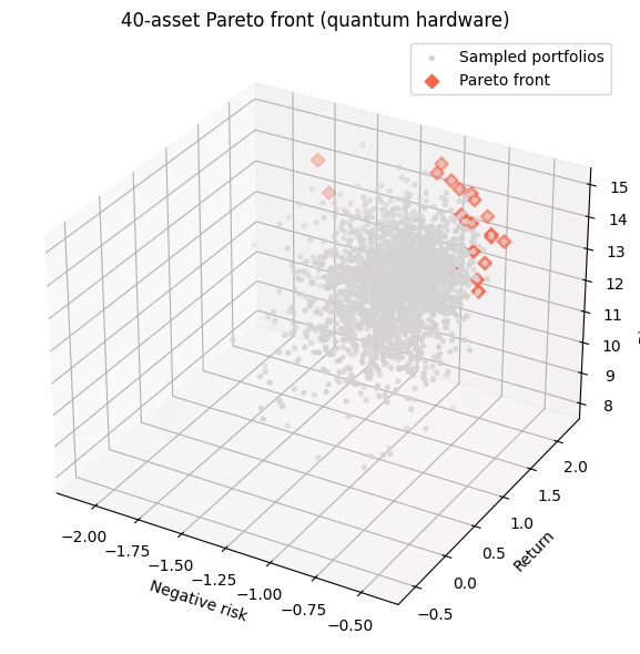
Feasible portfolios collected : 2359
Pareto-front portfolios       : 20

# --- Honest benchmark: QAOA and random vs the EXACT Pareto front ---
# 40 choose 6 = 3,838,380 feasible portfolios -- few enough to enumerate exactly, score
# every one on the TRUE objectives, and get the exact Pareto front. That front is an
# absolute ceiling, and its feasible nadir is a FIXED hypervolume reference point, so the
# numbers are comparable across runs instead of depending on what happened to be sampled.
import itertools

# Stream the combinations straight into an (n, K) index array, without first
# building millions of Python tuples.
combos = np.fromiter(
    itertools.chain.from_iterable(
        itertools.combinations(range(n_assets_40), K_40)
    ),
    dtype=np.int16,
).reshape(-1, K_40)
fis_exact = score_40(combos)
front_exact = filter_dominated(fis_exact, maximise=True)

# Fixed reference = worst value of each objective over ALL feasible portfolios (the nadir).
ref_fixed = fis_exact.min(axis=0)
# The hypervolume of a point set equals the hypervolume of its front.
hv_ceiling = hypervolume(front_exact, ref=ref_fixed, maximise=True)
hv_qaoa = hypervolume(fis_40, ref=ref_fixed, maximise=True)

def random_feasible_hv(n_draw, seed):
    """Hypervolume of n_draw uniformly-random feasible portfolios, same fixed reference."""
    rng = np.random.default_rng(seed)
    picks = set()
    while len(picks) < n_draw:
        picks.add(tuple(sorted(rng.choice(n_assets_40, K_40, replace=False))))
    P = np.array(list(picks))
    return hypervolume(score_40(P), ref=ref_fixed, maximise=True)

hv_rand = np.array(
    [random_feasible_hv(len(feasible_40), seed) for seed in range(20)]
)

print(f"Exact Pareto front            : {len(front_exact)} portfolios")
print(f"Hypervolume ceiling (optimum) : {hv_ceiling:.3f}")
print(
    f"QAOA (hardware)               : {100 * hv_qaoa / hv_ceiling:5.1f}% of optimum"
)
print(
    f"Random ({len(feasible_40)} draws, 20 seeds) : "
    f"{100 * hv_rand.mean() / hv_ceiling:5.1f}% +/- {100 * hv_rand.std() / hv_ceiling:.1f}% of optimum"
)

Exact Pareto front            : 61 portfolios
Hypervolume ceiling (optimum) : 64.211
QAOA (hardware)               :  85.5% of optimum
Random (2359 draws, 20 seeds) :  84.4% +/- 1.3% of optimum

ที่ขนาดปัญหานี้ QAOA ทำงานได้ดีพอๆ กับการสุ่มตัวอย่างแบบสุ่มสม่ำเสมอ ทั้งสองกู้คืน hypervolume ของค่าเหมาะสมที่สุดแบบแม่นตรงได้เป็นสัดส่วนมาก และไม่มีฝ่ายใดนำอย่างชัดเจน ผลลัพธ์นี้เป็นสิ่งที่คาดไว้สำหรับชั้น QAOA ตื้นชั้นเดียวที่มีตัวดำเนินการต้นทุนถูกตัดทอนมากบนฮาร์ดแวร์ที่มีสัญญาณรบกวน คุณค่าของตัวอย่างนี้คือเวิร์กโฟลว์หลายวัตถุประสงค์แบบครบวงจร (การแมป การฝึกมุม การสุ่มตัวอย่างแบบมีข้อจำกัด และการประมวลผลภายหลังแบบ Pareto) ไม่ใช่การเร่งความเร็วเชิงควอนตัม การลดช่องว่างกับค่าเหมาะสมที่สุดต้องใช้ circuit ที่ลึกขึ้น (ชั้น QAOA มากขึ้น) การตัดทอนที่นุ่มนวลกว่า หรือฮาร์ดแวร์ที่มีสัญญาณรบกวนต่ำกว่า

# The best trade-offs found by the sampler: no other sampled portfolio beats these
# on every objective. They approximate the exact front computed above; a
# decision-maker picks the trade-off they prefer.
bs_list = list(feasible_40)
# Boolean mask over fis_40; keep_weakly=True also keeps portfolios whose
# objective values tie with a front point (what the strict filter would drop).
mask = is_nondominated(fis_40, maximise=True, keep_weakly=True)
front_bs = [b for b, m in zip(bs_list, mask) if m]
front_f = fis_40[mask]
order = np.argsort(-front_f[:, 1])  # show a span sorted by return
print(
    f"{mask.sum()} non-dominated sampled portfolios. A representative span:\n"
)
print(
    f"{'tickers held':40s} {'risk':>7s} {'return':>7s} {'cross-sector':>12s}"
)
for idx in order[:: max(1, len(order) // 12)]:
    held = [tickers_40[i] for i, b in enumerate(front_bs[idx]) if b == "1"]
    print(
        f"{', '.join(held):40s} {-front_f[idx,0]:7.3f} {front_f[idx,1]:7.2f} {int(front_f[idx,2]):12d}"
    )

fig = plt.figure(figsize=(8, 6))
ax = fig.add_subplot(111, projection="3d")
ax.scatter(
    fis_40[:, 0],
    fis_40[:, 1],
    fis_40[:, 2],
    c="lightgray",
    s=8,
    label="Sampled portfolios",
)
ax.scatter(
    pareto_40[:, 0],
    pareto_40[:, 1],
    pareto_40[:, 2],
    c="tomato",
    marker="D",
    s=40,
    label="Pareto front",
)
ax.set_xlabel("Negative risk")
ax.set_ylabel("Return")
ax.set_zlabel("Diversification")
ax.set_title("40-asset Pareto front (quantum hardware)")
ax.legend()
plt.tight_layout()
plt.show()

20 non-dominated sampled portfolios. A representative span:

tickers held                                risk  return cross-sector
AAPL, NVDA, XOM, GS, BLK, CAT              1.715    2.22           13
NVDA, GS, MS, PFE, CAT, PLD                1.772    2.20           14
NVDA, MS, PFE, WMT, CAT, DUK               1.040    2.14           15
NVDA, CVX, GS, JNJ, KO, WMT                0.737    2.01           14
NVDA, COP, GS, JNJ, WMT, EQIX              1.014    1.98           15
NVDA, ABT, WMT, CAT, AEP, EQIX             0.913    1.92           15
NVDA, CVX, WMT, RTX, D, EQIX               0.835    1.82           15
NVDA, XOM, GS, JNJ, DUK, EQIX              0.763    1.80           15
AAPL, NVDA, JNJ, KO, RTX, SO               0.621    1.71           14
NVDA, CVX, BLK, JNJ, RTX, AEP              0.719    1.71           15
NVDA, JNJ, KO, COST, RTX, AEP              0.545    1.69           14
NVDA, CVX, ABT, WMT, HON, AEP              0.702    1.43           15
AAPL, GS, JNJ, PEP, AEP, EQIX              0.645    1.34           15
MSFT, XOM, BLK, JNJ, CAT, SO               0.617    1.34           15
MSFT, KO, WMT, RTX, SO, SPG                0.526    1.29           14
MSFT, XOM, BLK, JNJ, WMT, DUK              0.483    1.25           15
MSFT, CVX, JNJ, RTX, DUK, D                0.482    1.02           14
MSFT, XOM, JNJ, KO, HON, EQIX              0.479    0.93           15
MSFT, JNJ, PG, KO, RTX, DUK                0.423    0.86           14
MSFT, XOM, JNJ, PEP, DUK, AMT              0.476    0.57           15

ขั้นตอนถัดไป

คำแนะนำ

หากคุณสนใจบทเรียนนี้ ลองพิจารณาสิ่งต่อไปนี้:

• แทนที่ข้อมูลตลาดที่ดาวน์โหลด (market_data.csv) ด้วยค่าผลตอบแทนและค่าประมาณความแปรปรวนร่วมของคุณเองจากประวัติราคาจริง

• เพิ่มจำนวนชั้น QAOA หรือฝึกที่ 12–16 สินทรัพย์แล้วถ่ายโอนมุมเหล่านั้น เพื่อดันแนวหน้าบนฮาร์ดแวร์ให้เข้าใกล้ค่าเหมาะสมที่สุดมากขึ้น

• อ่าน Kotil et al., Quantum Approximate Multi-Objective Optimization (Nature Computational Science, 2025) งานศึกษา max-cut ที่บทเรียนนี้นำมาปรับใช้กับพอร์ตโฟลิโอ

เอกสารอ้างอิง

1. Kotil et al., "Quantum Approximate Multi-Objective Optimization," Nature Computational Science (2025). arXiv:2503.22797

2. S. H. Sack and M. Serbyn, "Quantum annealing initialization of the quantum approximate optimization algorithm," Quantum 5, 491 (2021). arXiv:2101.05742