เรียนรู้สถานะควอนตัมที่มีสัญญาณรบกวนด้วย classical shadows
ประมาณการใช้งาน: 34 นาทีบนตัวประมวลผล Heron r2 (หมายเหตุ: เป็นเพียงค่าประมาณ เวลาทำงานจริงของคุณอาจต่างออกไป)
ผลลัพธ์การเรียนรู้
-
เก็บการวัดแบบสุ่มบนตัวประมวลผลควอนตัม IBM® จาก Julia และบันทึกไว้สำหรับการวิเคราะห์ภายหลัง
-
ตรวจสอบข้อมูลการวัดหา qubit และ gate ที่บกพร่องก่อนเรียนรู้
-
ฟิตแบบจำลอง matrix product operator (MPO) ของสถานะที่มีสัญญาณรบกวนเข้ากับ classical shadows
-
ตรวจสอบแบบจำลองด้วยการวัดที่กันไว้ และเปรียบเทียบกับ circuit อุดมคติ
ความรู้พื้นฐานที่ต้องมี
-
Classical shadows ตามที่แนะนำในบทช่วยสอน Shadow tomography of the Greenberger-Horne-Zeilinger (GHZ) state
-
Density matrix และสถานะผสม ซึ่งครอบคลุมใน Basics of quantum information
-
การรัน circuit จาก Julia ด้วย
Qiskit.jlและQiskitIBMRuntime.jlซึ่งแนะนำในบทช่วยสอน Simulate time evolution of the transverse-field Ising model
ความเป็นมา
บนตัวประมวลผลควอนตัมจริง สัญญาณรบกวนเปลี่ยนสถานะบริสุทธิ์ ที่ circuit ถูกออกแบบมาเตรียมให้กลายเป็นสถานะผสม Full quantum state tomography สร้าง ขึ้นใหม่ได้ แต่จำนวนการวัดที่ต้องใช้เพิ่มขึ้นแบบเอกซ์โพเนนเชียลตามจำนวน qubit Votto และคณะ [1] จึงเรียนรู้แบบจำลองกะทัดรัดของ สำหรับสูงสุด 96 qubit จากการวัดแบบสุ่มแทน บทช่วยสอนนี้ทำตาม workflow ของพวกเขา
ในการวัดแบบสุ่ม [2] ทุก qubit ถูกหมุนด้วยยูนิทารีสุ่มอิสระ แล้ววัดในฐานการคำนวณ การสุ่มการหมุนหนึ่งครั้งเรียกว่า measurement setting และแต่ละ setting ถูกทำซ้ำ shot shot ที่ได้บิตผลลัพธ์ ให้ classical shadow [3]
ซึ่งค่าเฉลี่ยของมันเหนือ setting และ shot คือ บทช่วยสอนที่เป็นความรู้พื้นฐานสุ่ม แต่ละตัวจากฐาน Pauli สามฐาน บทช่วยสอนนี้เหมือนกับในบทความ คือสุ่มอย่างสม่ำเสมอจากยูนิทารีหนึ่ง qubit ทั้งหมด (Haar random) และสูตรเดิมใช้ได้เหมือนกัน
Shadow ประมาณสมบัติของ qubit ไม่กี่ตัวต่อครั้ง บทความรวมมันเป็น matrix product operator (MPO) ซึ่งเขียน density matrix เป็นโซ่ของเทนเซอร์ขนาดเล็ก หนึ่งตัวต่อ qubit สถานะที่มีสัญญาณรบกวนและสหสัมพันธ์ระยะสั้นต้องการ bond เล็กระหว่างเทนเซอร์ข้างเคียงเท่านั้น เช่นเดียวกับอัลกอริทึม density matrix renormalization group (DMRG) ตัวเรียนรู้กวาดไปตามโซ่และอัปเดตเทนเซอร์ทีละตัว เพื่อให้แบบจำลองตรงกับ shadow บนหน้าต่าง qubit ที่อยู่กึ่งกลางเทนเซอร์นั้น (สมการที่ 4 ของบทความ) bond dimension คงที่ระหว่างการอัปเดตเหล่านี้ ตัวเรียนรู้จึงไม่ตัดทอนแบบจำลองเลย เนื่องจากข้อมูลเข้ามาผ่านหน้าต่างเหล่านี้เท่านั้น จำนวน setting ที่ต้องใช้จึงไม่เพิ่มตามความยาวของโซ่
setting ถูกแบ่งเป็นชุดฝึกและชุดทดสอบ บนชุดทดสอบ บทความประมาณ max fidelity ระหว่าง กับแบบจำลอง
การวัด โดยตรงต้องใช้การวัดจำนวนมหาศาลแบบเอกซ์โพเนนเชียล บทความจึงสมมติ approximate factorization condition (AFC) แทน คือสหสัมพันธ์ใน ลดลงภายในไม่กี่ qubit ดังนั้น overlap และ purity ระดับโลกแยกตัวประกอบเป็นพจน์บนบล็อก qubit ที่อยู่ติดกัน purity ยังให้ Rényi-2 entropy ซึ่งวัดว่าสถานะผสมมากแค่ไหน
บทความเตรียมสถานะ kicked-Ising ความลึก
บน 96 qubit ของ ibm_brisbane ซึ่งเป็นตัวประมวลผล Eagle ด้วย 2,048 setting ที่มี 1,024 shot สำหรับ รูปที่ 1(c,d) ของบทความรายงานสองผลลัพธ์สำหรับ :
-
แบบจำลองที่เรียนรู้ได้ กับสถานะจากการทดลองที่ สูงกว่า overlap ของสถานะอุดมคติ กับการทดลองมาก
-
เอนโทรปีเพิ่มขึ้นเชิงเส้น และเอนโทรปีของแบบจำลองสอดคล้องกับค่าประมาณอิสระจากชุดทดสอบ
บทช่วยสอนนี้ตรวจสอบทั้งสองผลลัพธ์ ก่อนในการจำลองแปด qubit ที่ทราบคำตอบที่แน่นอน แล้วจึงในการรันใหม่ 96 qubit บน ibm_fez ซึ่งเป็นตัวประมวลผล Heron r2 ตัวเรียนรู้เป็นการนำสมการในบทความและภาคผนวกไปใช้ใน Julia แบบอิสระ
ข้อกำหนด
บทช่วยสอนนี้ต้องใช้ macOS หรือ Linux เพราะ Qiskit.jl ยังไม่รองรับ Windows (Qiskit.jl issue #15) คุณยังต้องมีสิ่งต่อไปนี้:
-
Julia 1.11 จาก หน้าดาวน์โหลด Julia หรือด้วย
juliaup add 1.11และแพ็กเกจIJulia:julia -e 'using Pkg; Pkg.add("IJulia")' -
สำหรับตัวอย่างบนฮาร์ดแวร์ ต้องมี บัญชี IBM Quantum® Platform ที่เข้าถึง QPU ที่มีอย่างน้อย 96 qubit และ credentials ที่บันทึกไว้ หากไม่มีบัญชี คุณรันตัวอย่างบนฮาร์ดแวร์ได้จากการวัดที่บันทึกไว้ของการรัน
ibm_fezที่ให้ผลลัพธ์ในบทช่วยสอนนี้ ส่วนอื่นรันได้โดยไม่ต้องมีบัญชี
notebook ใช้ Qiskit.jl และ QiskitIBMRuntime.jl เพื่อสร้างและรัน circuit ใช้ RandomMeas.jl [4] สำหรับการวัดแบบสุ่ม (ซึ่งมี ITensors.jl และ ITensorMPS.jl ให้ด้วย) และ NPZ.jl, JSON.jl และ Plots.jl บทช่วยสอนนี้ทดสอบกับ Qiskit.jl 0.6.1, QiskitIBMRuntime.jl 0.3.2 และ RandomMeas.jl 0.3.1
มีสองวิธีในการตั้งค่าสภาพแวดล้อม:
-
ตัวเลือก 1: ติดตั้งแพ็กเกจเวอร์ชันล่าสุดที่เข้ากันได้ลงในสภาพแวดล้อมชั่วคราว รันเซลล์ต่อไปนี้โดยไม่ต้องแก้ไข
-
ตัวเลือก 2: ทำซ้ำสภาพแวดล้อมที่ทดสอบแบบตรงทุกประการ ตั้ง
download_toml_files = trueในเซลล์ต่อไปนี้ เซลล์จะดาวน์โหลดProject.tomlและManifest.tomlจาก repository เอกสาร ไปไว้ในโฟลเดอร์env_tutorial/classical-shadows/ข้าง notebook นี้ แล้วติดตั้งเวอร์ชันที่แน่นอนของทุกแพ็กเกจที่ manifest บันทึกไว้ รวมถึง dependency ทางอ้อม สำหรับรายละเอียด ดู เอกสาร Julia เกี่ยวกับไฟล์เหล่านี้
using Pkg
using Downloads

download_toml_files = false

if !download_toml_files
    # Option 1: Install the latest compatible versions into a temporary environment
    Pkg.activate(mktempdir(); io=devnull)
    Pkg.add([
        PackageSpec(name="Qiskit", version="0.6"),
        PackageSpec(name="QiskitIBMRuntime", version="0.3"),
        PackageSpec(name="RandomMeas", version="0.3"),
        PackageSpec(name="NPZ"),
        PackageSpec(name="JSON"),
        PackageSpec(name="Plots"),
    ]; io=devnull)
else
    # Option 2: Install the exact tested versions recorded in Project.toml and Manifest.toml
    base_url = "https://raw.githubusercontent.com/Qiskit/documentation/main/docs/tutorials/assets/classical-shadows/julia"
    env_dir = joinpath(@__DIR__, "env_tutorial", "classical-shadows")
    mkpath(env_dir)
    for file in ("Project.toml", "Manifest.toml")
        Downloads.download("$base_url/$file", joinpath(env_dir, file))
    end
    Pkg.activate(env_dir; io=devnull)
    Pkg.instantiate(; io=devnull)
end
การตั้งค่า
using RandomMeas  # also loads ITensors and ITensorMPS
using Qiskit, QiskitIBMRuntime
using Random, LinearAlgebra, Statistics
using Downloads, SHA, NPZ, JSON, Plots

# Download the helper module that implements the learner, unless a copy exists
docs_url = "https://raw.githubusercontent.com/Qiskit/documentation/main"
helper_file = joinpath(@__DIR__, "env_tutorial", "classical-shadows", "mpo_learning.jl")
if !isfile(helper_file)
    mkpath(dirname(helper_file))
    helper_url = "$docs_url/docs/tutorials/assets/classical-shadows/julia/mpo_learning.jl"
    Downloads.download(helper_url, helper_file)
end
include(helper_file)
using .ShadowMPOLearning
BLAS.set_num_threads(1)  # the learner multiplies many small matrices
โมดูลตัวช่วย mpo_learning.jl ซึ่งเซลล์ Setup ดาวน์โหลด เป็นตัวนำตัวเรียนรู้ไปใช้ บทช่วยสอนเรียกฟังก์ชันต่อไปนี้จากมัน:
| ฟังก์ชัน | วัตถุประสงค์ |
|---|---|
kicked_ising_reference(N, D; depolarization) | MPO ที่แน่นอนของสถานะ kicked-Ising อุดมคติ หรือของสถานะหลังสัญญาณรบกวน depolarizing เฉพาะที่ |
split_settings(group; seed, train_fraction) | กำหนด measurement setting เข้าชุดฝึกและชุดทดสอบแบบสุ่ม (ชุดละครึ่งโดยค่าเริ่มต้น) |
training_marginals(train; ell, prior) | ค่าประมาณ shadow ของทุกหน้าต่างการเรียนรู้ จาก setting ของชุดฝึกเท่านั้น |
fitted_prior(ideal, train) | Prior สำหรับ common randomized measurements (CRM) ที่ฟิตกับ purity ที่วัดได้ของแต่ละหน้าต่าง ตามบทความ |
learn_mpo(marginals, N; ell, maxbond, sweeps) | กวาดการอัปเดตหนึ่งไซต์ของบทความไปตามโซ่ โดยเริ่มจากสถานะผสมสูงสุด |
max_fidelity(a, b), mpo_overlap(a, b) | และ ที่แน่นอนระหว่างสอง MPO |
afc_estimate, afc_statistics, afc_prefix_curve | ค่าประมาณ AFC ของ และ จาก setting ของชุดทดสอบ พร้อมแถบความคลาดเคลื่อนแบบ jackknife |
ตัวเรียนรู้เก็บ MPO ในฐาน Pauli ซึ่งทำให้แบบจำลองเป็น Hermitian และมี trace หนึ่ง แต่ไม่บังคับให้แบบจำลองเป็น positive semidefinite ดังนั้น notebook จึงรายงานว่าค่าไอเกนติดลบแค่ไหน
ตัวอย่างตัวจำลองขนาดเล็ก
เริ่มจากระบบที่เล็กพอจะคำนวณทุกอย่างได้แน่นอน คือสถานะ kicked-Ising ความลึกหนึ่งบนแปด qubit พร้อมสัญญาณรบกวน depolarizing เฉพาะที่ 12% เพื่อจำลองฮาร์ดแวร์ เนื่องจากทราบสถานะที่มีสัญญาณรบกวน คุณจึงเปรียบเทียบแบบจำลองที่เรียนรู้กับมันได้โดยตรง
ขั้นตอนที่ 1: แมปอินพุตคลาสสิกเป็นปัญหาควอนตัม
ฟังก์ชัน kicked_ising_reference คืนสถานะที่แน่นอนเป็น MPO เมื่อ depolarization=0.12 เวกเตอร์ Bloch ของทุก qubit จะหดลง 12% หลัง circuit
N = 8
ideal = kicked_ising_reference(N, 1)
rho = kicked_ising_reference(N, 1; depolarization=0.12)
println("Purity of the noisy state: ", round(mpo_overlap(rho, rho), digits=3))
println("F_max between the noisy and ideal states: ", round(max_fidelity(rho, ideal), digits=3))
Purity of the noisy state: 0.327
F_max between the noisy and ideal states: 0.56
ขั้นตอนที่ 2: ปรับปัญหาให้เหมาะกับการรันบนฮาร์ดแวร์ควอนตัม
ตัวอย่างนี้สุ่มผลการวัดแบบคลาสสิก จึงไม่มี circuit ให้ transpile ตัวอย่างบนฮาร์ดแวร์ครอบคลุมขั้นตอนนี้
ขั้นตอนที่ 3: รันโดยใช้ Qiskit primitives
ใช้ RandomMeas.jl สุ่ม measurement setting แบบ Haar-random 2,048 ชุด และสุ่ม 256 shot จากแต่ละชุด แล้วแบ่ง setting เท่า ๆ กันเป็นชุดฝึกและชุดทดสอบ แบ่งตาม setting ไม่ใช่ตาม shot เพราะ shot จาก setting เดียวกันใช้การหมุนร่วมกัน จึงไม่เป็นอิสระต่อกัน
Random.seed!(20260921)
sites = siteinds("Qubit", N)
settings = [LocalUnitaryMeasurementSetting(N; site_indices=sites, ensemble=Haar) for _ in 1:2048]
measurements = MeasurementGroup(to_itensor_mpo(rho, sites), settings, 256)
split = split_settings(measurements; seed=20260921)
println(length(split.train_ids), " training settings, ", length(split.test_ids), " testing settings")
1024 training settings,
1024 testing settings
ขั้นตอนที่ 4: ประมวลผลหลังการวัดและส่งคืนผลลัพธ์ในรูปแบบคลาสสิกที่ต้องการ
เรียนรู้แบบจำลองด้วยพารามิเตอร์ความลึกหนึ่งของบทความ คือหน้าต่างที่ขยาย qubit ทั้งสองข้างของเทนเซอร์ที่อัปเดต bond dimension 4 และ 20 sweep เริ่มจากสถานะผสมสูงสุด sweep แรกอัปเดตคู่เทนเซอร์ข้างเคียง ซึ่งทำให้ bond dimension เพิ่มจาก 1 เป็น 4 ทุก sweep ถัดไปอัปเดตเทนเซอร์ทีละตัวที่ bond dimension คงที่นั้น
เพื่อลดสัญญาณรบกวนทางสถิติของ shadow บทความใช้ common randomized measurements (CRM) [5] สำหรับแต่ละ setting มันลบ shadow เฉลี่ยที่การคาดเดาสถานะล่วงหน้า (prior) จะสร้างใน setting เดียวกัน แล้วบวกค่าที่แน่นอนของ prior กลับเข้าไป การแก้ไขนี้เฉลี่ยเป็นศูนย์ ดังนั้น prior เปลี่ยนขนาดของความคลาดเคลื่อนทางสถิติแต่ไม่เปลี่ยนสิ่งที่ถูกประมาณ ในที่นี้ prior คือสถานะอุดมคติที่มี depolarization เฉพาะที่ 10% ใกล้เคียง 12% ที่แท้จริง บนฮาร์ดแวร์ ระดับสัญญาณรบกวนไม่ทราบ ตัวอย่างบนฮาร์ดแวร์จึงฟิต prior กับ purity ที่วัดได้แทน ตามที่บทความทำ
prior = kicked_ising_reference(N, 1; depolarization=0.10)
marginals = training_marginals(split.train; ell=2, prior)
fit = learn_mpo(marginals, N; ell=2, maxbond=4, sweeps=20)
sigma = fit.model
plot([h.sweep for h in fit.history], [h.local_loss for h in fit.history];
    xlabel="sweep", ylabel="mean squared residual", label="training windows",
    size=(680, 320), left_margin=5Plots.mm, bottom_margin=5Plots.mm)
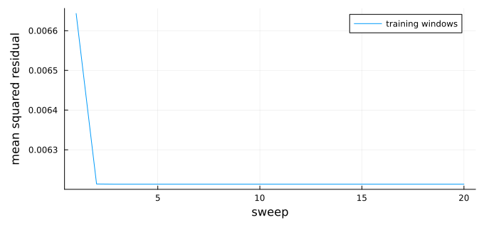
residual วัดว่าหน้าต่างของแบบจำลองห่างจาก shadow ของชุดฝึกแค่ไหน มันลดลงเมื่อการอัปเดตหนึ่งไซต์เริ่มใน sweep ที่สอง แล้วคงที่โดยประมาณแทนที่จะถึงศูนย์ เพราะ shadow มีสัญญาณรบกวนทางสถิติที่แบบจำลองที่มี bond dimension เล็กสร้างซ้ำไม่ได้
เนื่องจากทราบสถานะนี้ คุณจึงเปรียบเทียบแบบจำลองที่เรียนรู้กับมันได้อย่างแน่นอน และเปรียบเทียบกับการคาดเดาที่ง่ายที่สุดสองแบบด้วย คือ CRM prior และสถานะอุดมคติ
eigenvalues = eigvals(Hermitian(dense_operator(sigma)))
println("F_max with the noisy state")
println("  learned model: ", round(max_fidelity(rho, sigma), digits=3))
println("  CRM prior:     ", round(max_fidelity(rho, prior), digits=3))
println("  ideal state:   ", round(max_fidelity(rho, ideal), digits=3))
println("Most negative eigenvalue of the model: ", round(minimum(eigenvalues), digits=4))
println("Total negative eigenvalue weight:      ", round(-sum(min.(eigenvalues, 0)), digits=4))
F_max with the noisy state
learned model: 0.993
  CRM prior:     0.911
  ideal state:   0.56
Most negative eigenvalue of the model: -0.0076
Total negative eigenvalue weight:      0.0348
แบบจำลองที่เรียนรู้ใกล้สถานะที่มีสัญญาณรบกวนมากกว่าทั้ง prior และสถานะอุดมคติ จึงเรียนรู้สัญญาณรบกวนจากข้อมูลได้ ค่าไอเกนติดลบเล็กน้อยของมันมาจากจำนวนการวัดที่จำกัด
บนฮาร์ดแวร์ ไม่ทราบสถานะ คุณจึงประมาณ จาก setting ของชุดทดสอบแทน AFC แบ่งโซ่เป็นบล็อก ละ qubit และประมาณ purity ด้วย
และ ด้วยอัตราส่วนเดียวกันของ overlap เฉพาะที่ เมื่อ สองบล็อกครอบคลุมทั้งแปด qubit และสูตรแม่นยำ เมื่อ สูตรพึ่งสมมติฐานการแยกตัวประกอบ แถบความคลาดเคลื่อนแบบ jackknife ซึ่งตัด setting ของชุดทดสอบออกทีละตัว ครอบคลุมความคลาดเคลื่อนทางสถิติของข้อมูลชุดทดสอบเท่านั้น ไม่รวมความสุ่มของการฝึกหรือการประมาณ AFC
for k in (2, 4)
    estimate = afc_estimate(sigma, split.test; k, statistics=afc_statistics(split.test, k; prior))
    println("k = $k: held-out F_max = ", round(estimate.fidelity, digits=3), " ± ",
        round(estimate.fidelity_sem, digits=3))
end
println("Exact F_max:              ", round(max_fidelity(rho, sigma), digits=3))
k = 2: held-out F_max = 0.966
± 0.036
k = 4: held-out F_max =
0.958 ± 0.049
Exact F_max:              0.993
ค่าประมาณจากข้อมูลที่กันไว้ทั้งสองสอดคล้องกับค่าที่แน่นอนภายในแถบความคลาดเคลื่อน
ตัวอย่างบนฮาร์ดแวร์ขนาดใหญ่
ตอนนี้รันการทดลองบนโซ่ 96 qubit ของ ibm_fez ซึ่งเป็นตัวประมวลผล Heron r2 เหมือน ibm_brisbane มันมี coupling map แบบ heavy-hex และระดับสัญญาณรบกวนใกล้เคียงกัน
การเก็บข้อมูลใช้ Sampler job 1,024 รายการและเวลา QPU ประมาณ 34 นาที ถ้าคุณไม่มีสิทธิ์เข้าถึง QPU ที่มีอย่างน้อย 96 qubit หรือคิวยาว ให้รันตัวอย่างบนฮาร์ดแวร์จากการวัดที่บันทึกไว้บน ibm_fez เมื่อวันที่ 27 กันยายน 2026 ซึ่งให้ผลลัพธ์ที่แสดงในบทเรียนนี้ เมื่อตั้ง use_saved_data = true โน้ตบุ๊กจะดาวน์โหลดการวัดเหล่านี้ (15 MB) จาก Zenodo [6] ในขั้นตอนที่ 1 และข้ามการส่ง job ในขั้นตอนที่ 3 หากต้องการเก็บข้อมูลของคุณเอง ให้ตั้งเป็น false
use_saved_data = true; # set to false to collect new measurements on hardware
ขั้นตอนที่ 1: แมปอินพุตคลาสสิกเป็นปัญหาควอนตัม
แต่ละการตั้งค่าต้องใช้ circuit หนึ่งตัว ได้แก่ kicked-Ising circuit, Gate บนแต่ละ qubit สำหรับ และการวัดทุก qubit การสุ่ม โดยที่ , และ กระจายสม่ำเสมอใน ทำให้ เป็น Haar random ฟังก์ชัน u3_matrix คืนค่าเมทริกซ์ของ ซึ่งขั้นตอนที่ 4 ใช้งาน
งบประมาณคือ 1,024 การตั้งค่า การตั้งค่าละ 1,024 shot ซึ่งเป็นครึ่งหนึ่งของจำนวนการตั้งค่าในเปเปอร์ แบ่งเท่า ๆ กันระหว่างการฝึกและการทดสอบ เมื่อใช้ข้อมูลที่บันทึกไว้ เซลล์จะโหลดมุมที่บันทึกไว้ มิฉะนั้นจะสุ่มมุมใหม่และบันทึกก่อนที่คุณจะส่งอะไรก็ตาม เพราะคุณวิเคราะห์ผลลัพธ์ไม่ได้ถ้าไม่มีมุมเหล่านั้น ถ้าไฟล์มีอยู่แล้ว เซลล์จะโหลดไฟล์นั้น เพื่อให้มุมยังตรงกับผลลัพธ์ที่บันทึกไว้หลังจากคุณรีสตาร์ท Session
"Matrix of the U(θ, ϕ, λ) gate, as used by `qc.u` in Qiskit."
u3_matrix(θ, ϕ, λ) = [cos(θ/2)              -exp(im*λ)*sin(θ/2);
                      exp(im*ϕ)*sin(θ/2)    exp(im*(ϕ + λ))*cos(θ/2)]

"Angles (θ, ϕ, λ) for which `u3_matrix(θ, ϕ, λ)` is a Haar-random unitary."
random_u3_angles() = (2asin(sqrt(rand())), 2π*rand(), 2π*rand())

N_hw, NU_hw, NM_hw = 96, 1024, 1024
data_directory = joinpath(@__DIR__, "classical-shadows-data")
saved_file = joinpath(data_directory, "ibm-fez-run.npz")
run_directory = joinpath(data_directory, "new-run")
settings_file = joinpath(run_directory, "settings.npz")
if use_saved_data
    saved_url = "https://zenodo.org/records/24116174/files/ibm-fez-run.npz?download=1"
    saved_sha256 = "c42f4d8d42e5083e9e152b4fec0846884ebe3be003e5ab528deebf4f00c9fe50"
    if !isfile(saved_file)
        mkpath(data_directory)
        println("Downloading the saved ibm_fez run (15 MB)...")
        Downloads.download(saved_url, saved_file * ".part")
        mv(saved_file * ".part", saved_file)
    end
    bytes2hex(open(sha256, saved_file)) == saved_sha256 ||
        error("$saved_file is incomplete or corrupted; delete it and run this cell again")
    saved_run = npzread(saved_file)
    angles = saved_run["angles"]
elseif isfile(settings_file)
    angles = npzread(settings_file)["angles"]
else
    mkpath(joinpath(run_directory, "outcomes"))
    Random.seed!(20260927)
    angles = Array{Float64}(undef, NU_hw, N_hw, 3)
    for r in 1:NU_hw, i in 1:N_hw
        angles[r, i, :] .= random_u3_angles()
    end
    npzwrite(settings_file, Dict("angles" => angles))
end
println("Measurement settings: ", size(angles, 1), " × ", size(angles, 2), " qubits")
Measurement settings: 1024
× 96 qubits
ขั้นตอนที่ 2: ปรับปัญหาให้เหมาะสมสำหรับการรันบนฮาร์ดแวร์ควอนตัม
โซ่จะดีได้แค่ qubit ที่แย่ที่สุด ดังนั้นให้เลือก physical qubit 96 ตัวด้วยตัวเอง ฟังก์ชัน transpile ของ Qiskit.jl ยังไม่รองรับ initial layout แบบกำหนดตายตัว และในการทดสอบบน ibm_phoenix layout ที่มันเลือกมี qubit ที่มี readout error 51% โซ่ต่อไปนี้คือเส้นทาง 96 qubit ใน coupling map ของ ibm_fez ที่ layout แบบคำนึงถึงข้อผิดพลาดของฟังก์ชัน transpile ใน Python Qiskit (ด้วย optimization_level=3) เลือกจากข้อมูลการสอบเทียบของวันที่ 27 กันยายน 2026 readout error เฉลี่ยของมันคือ 1.6% แต่แลตทิซ heavy-hex มีเส้นทาง 96 qubit น้อยมาก และเส้นนี้มี qubit 35 ซึ่งมี readout error 15% การสอบเทียบเปลี่ยนแปลงได้ ดังนั้นให้เลือกโซ่ใหม่จากข้อมูลการสอบเทียบปัจจุบันก่อนรันในวันอื่นหรือบน QPU อื่น
เพื่อคงโซ่นี้ไว้ ให้เขียน circuit โดยตรงด้วย native gate แทนการ transpile Gate เท่ากับ จนถึงเฟสรวม การแยกส่วนนี้ครอบคลุมทั้งการหมุนแบบสุ่มและ kick Gate เท่ากับ CZ gate ตามด้วย บน qubit ทั้งสองตัว จนถึงเฟสรวม เนื่องจาก gate เหล่านี้เป็นแนวทแยง จึงสลับที่กับ CZ gate ได้ ดังนั้นแต่ละ qubit จะสะสม หนึ่งตัวต่อหนึ่งพันธะก่อนการหมุนเพื่อวัด
num_device_qubits = 156
# Physical qubits of ibm_fez, in IBM numbering, forming the chain
chain_physical = [
    2, 3, 4, 5, 6, 7, 8, 9, 10, 11, 12, 13, 14, 15, 19, 35, 34, 33, 39, 53, 54, 55, 59, 75, 74,
    73, 79, 93, 94, 95, 99, 115, 114, 113, 119, 133, 132, 131, 130, 129, 128, 127, 137, 147, 146,
    145, 144, 143, 136, 123, 124, 125, 117, 105, 106, 107, 108, 109, 110, 111, 98, 91, 90, 89,
    88, 87, 86, 85, 77, 65, 66, 67, 68, 69, 70, 71, 58, 51, 50, 49, 48, 47, 46, 45, 37, 25, 24,
    23, 22, 21, 36, 41, 42, 43, 56, 63]
chain = chain_physical .+ 1  # Qiskit.jl numbers qubits from 1

"Apply U(θ, ϕ, λ) to qubit q with native gates: rz(λ), sx, rz(θ + π), sx, rz(ϕ + π)."
function native_u!(qc, q, θ, ϕ, λ)
    qc.rz(λ, q)
    qc.sx(q)
    qc.rz(θ + π, q)
    qc.sx(q)
    qc.rz(ϕ + π, q)
end

"Kicked-Ising circuit on `chain`, then the rotations of one setting and a measurement."
function native_setting_circuit(chain, angles, num_device_qubits)
    n = length(chain)
    qc = QuantumCircuit(num_device_qubits, n)
    for q in chain
        native_u!(qc, q, π/4, -π/2, π/2)       # e^{-iπ/8 X}
    end
    for i in 1:n-1
        qc.cz(chain[i], chain[i + 1])          # e^{iπ/4 ZZ}, up to the S† gates below
    end
    for (i, q) in enumerate(chain)
        bonds = (i > 1) + (i < n)
        qc.rz(-π/2 * bonds, q)                 # one S† per bond
        native_u!(qc, q, angles[i, 1], angles[i, 2], angles[i, 3])
        qc.measure(q, i)                       # outcome of chain qubit i goes to bit i
    end
    qc
end

circuits = [native_setting_circuit(chain, angles[r, :, :], num_device_qubits) for r in 1:NU_hw]
println(length(circuits), " circuits, each with ", count(inst -> inst.name == "cz", circuits[1].data), " CZ gates")
1024 circuits, each with
95 CZ gates
ขั้นตอนที่ 3: รันโดยใช้ Qiskit primitive
QiskitIBMRuntime.jl รันหนึ่ง circuit ต่อหนึ่ง Sampler job ดังนั้นการเก็บข้อมูลต้องใช้ 1,024 job เซลล์ต่อไปนี้เก็บ job ไว้ในคิวได้สูงสุด 32 รายการ และบันทึกผลลัพธ์ของแต่ละการตั้งค่าทันทีที่ job เสร็จ แต่ละ shot จะถูกคืนค่าเป็นเวกเตอร์ของบิต โดยที่องค์ประกอบ คือผลลัพธ์ของ qubit ลำดับที่ ในโซ่
คุณต้องดึงผลลัพธ์ใน Session เดียวกับที่ส่ง job เพราะ QiskitIBMRuntime.jl ยังค้นหา job ด้วย ID ไม่ได้ (qiskit-ibm-runtime-c issue #28) ถ้า job ล้มเหลว เซลล์จะแสดงคำเตือนแล้วทำงานต่อ ถ้า Session หยุด ให้รันขั้นตอนที่ 1 ถึง 3 ใหม่ การรันเซลล์ซ้ำจะส่งเฉพาะการตั้งค่าที่ยังไม่มีผลลัพธ์ เมื่อ use_saved_data = true เซลล์จะไม่ส่งอะไรเลย
outcome_file(r) = joinpath(run_directory, "outcomes", "setting_$(lpad(r, 4, '0')).npz")

"Save the outcomes of setting `r` as a (shots × N) matrix of 0/1 values."
function save_outcomes(r, job)
    try
        samples = get_sampler_job_results(job, service)
        bits = UInt8.(permutedims(reduce(hcat, samples)))
        npzwrite(outcome_file(r), Dict("bits" => bits))
    catch err
        @warn "Setting $r failed and was not saved; run this cell again to resubmit it" err
    end
end

if use_saved_data
    println("Using the saved ibm_fez measurements; no jobs submitted")
else
    backend_name = "ibm_fez"
    service = Service()  # uses the credentials saved on this computer
    backend = only(b for b in backend_search(service) if b.name == backend_name)
    open(joinpath(run_directory, "metadata.json"), "w") do io
        JSON.print(io, Dict("backend" => backend_name, "N" => N_hw, "depth" => 1, "settings" => NU_hw,
                            "shots" => NM_hw, "chain" => chain_physical), 2)
    end
    in_flight = []
    for r in 1:NU_hw
        isfile(outcome_file(r)) && continue
        push!(in_flight, (r, run_sampler_job(service, backend, circuits[r], NM_hw)))
        length(in_flight) >= 32 && save_outcomes(popfirst!(in_flight)...)
    end
    foreach(job -> save_outcomes(job...), in_flight)
    println("Saved outcomes: ", count(r -> isfile(outcome_file(r)), 1:NU_hw), " of ", NU_hw, " settings")
end
Using the saved ibm_fez measurements; no jobs submitted
ขั้นตอนที่ 4: ประมวลผลหลังการรันและคืนผลลัพธ์ในรูปแบบคลาสสิกที่ต้องการ
ขั้นตอนนี้อ่านเฉพาะข้อมูลที่บันทึกไว้ ได้แก่ การรัน ibm_fez ที่ดาวน์โหลดมาถ้า use_saved_data เป็น true หรือไฟล์ที่ขั้นตอนที่ 3 เขียนไว้ในกรณีอื่น ดังนั้นคุณจึงรันขั้นตอนนี้ใน Session ใหม่ได้โดยไม่ต้องส่ง job (รันเซลล์ Setup, เซลล์ use_saved_data และขั้นตอนที่ 1 ก่อน) ไฟล์ที่ดาวน์โหลดเก็บผลลัพธ์ 96 บิตของแต่ละ shot อัดเป็น 12 ไบต์ โดยเรียงบิตที่มีนัยสำคัญสูงสุดก่อน ตัวโหลดจึงต้องแตกข้อมูลออก RandomMeas.jl ระบุผลลัพธ์เป็น 1 และ 2 ตัวโหลดจึงบวก 1 ให้ทุกบิตด้วย
"Build a `MeasurementGroup` from the angles and a function `outcomes(r)` that returns
the (shots × N) 0/1 outcomes of setting `r`."
function measurement_group(angles, outcomes)
    settings_count, n = size(angles, 1), size(angles, 2)
    sites = siteinds("Qubit", n)
    data = map(1:settings_count) do r
        rotations = Array{ComplexF64}(undef, n, 2, 2)
        for i in 1:n
            rotations[i, :, :] = u3_matrix(angles[r, i, :]...)
        end
        MeasurementData(Int.(outcomes(r)) .+ 1;
            measurement_setting=LocalUnitaryMeasurementSetting(rotations; site_indices=sites))
    end
    MeasurementGroup(data)
end

if use_saved_data
    packed = saved_run["outcomes"]  # settings × shots × 12 bytes
    # Bit i of a shot is in byte (i - 1) ÷ 8 + 1, most significant bit first
    unpack(r) = [(packed[r, s, (i - 1) ÷ 8 + 1] >> (7 - (i - 1) % 8)) & 0x01
                 for s in 1:size(packed, 2), i in 1:N_hw]
    group_hw = measurement_group(angles, unpack)
else
    group_hw = measurement_group(angles, r -> npzread(outcome_file(r))["bits"])
end
println(group_hw.NU, " settings × ", group_hw.NM, " shots on ", group_hw.N, " qubits")
1024 settings ×
1024 shots on 96 qubits
ก่อนเรียนรู้ ให้ตรวจสอบข้อมูล qubit ที่เสียหรือ Gate ที่สอบเทียบไม่ดีทำให้สถานะที่วัดได้รอบ ๆ มันผสมมากขึ้นมาก และอาจทำให้ตัวเรียนรู้ไม่ลู่เข้า purity ของ qubit ข้างเคียงสองสามตัวเป็นเกณฑ์วัดสัญญาณรบกวนนี้แบบไม่ขึ้นกับโมเดล ฟังก์ชัน get_purity จาก RandomMeas.jl ประมาณค่า สำหรับระบบย่อย โดยเปรียบเทียบคู่ของ shot จากการตั้งค่าเดียวกัน คำนวณเอนโทรปี Rényi-2 ของทุกหน้าต่างที่มี qubit ข้างเคียงหกตัว แล้วเปรียบเทียบกับหน้าต่างเดียวกันของสถานะอุดมคติ ค่าอุดมคติไม่ใช่ศูนย์ เพราะแต่ละหน้าต่างพันกันกับส่วนที่เหลือของโซ่ สัญญาณรบกวนทำให้ค่านี้เพิ่มขึ้น และ qubit ที่เสียจะดันทุกหน้าต่างที่มันอยู่ไปทางค่าสูงสุดคือหก
ideal_hw = kicked_ising_reference(N_hw, 1)
width = 6
starts = 1:N_hw - width + 1
window_entropy(rho, w) = -log2(mpo_overlap(segment_mpo(rho, w), segment_mpo(rho, w)))
measured_entropy = [-log2(get_purity(group_hw, collect(j:j + width - 1))) for j in starts]
ideal_entropy = [window_entropy(ideal_hw, j:j + width - 1) for j in starts]
worst = argmax(measured_entropy)
println("S₂ of six-qubit windows: median ", round(median(measured_entropy), digits=2), "; highest ",
    round(measured_entropy[worst], digits=2), " (chain positions ", worst, " to ", worst + width - 1, ")")
println("Ideal state: ", round(minimum(ideal_entropy), digits=2), " to ", round(maximum(ideal_entropy), digits=2))
plot(starts, measured_entropy; marker=:circle, markersize=2, label="measured",
    xlabel="first chain position of the window", ylabel="S₂ of six qubits", ylims=(0, width),
    legend=:topright, size=(800, 280), left_margin=5Plots.mm, bottom_margin=5Plots.mm)
plot!(starts, ideal_entropy; linestyle=:dash, label="ideal state")
S₂ of six-qubit windows: median 0.9
; highest 1.43 (chain positions 30 to 35)
Ideal state: 0.19 to 0.39
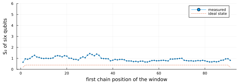
ทุกหน้าต่างผสมมากกว่าสถานะอุดมคติ ประมาณครึ่งบิตถึงหนึ่งบิต และช่วงที่มีสัญญาณรบกวนมากที่สุดอยู่รอบตำแหน่ง 30 ถึง 35 ในโซ่ ไม่มีหน้าต่างใดใกล้ค่าสูงสุดคือหก ดังนั้นไม่มี qubit ที่เสีย และการวิเคราะห์ใช้โซ่ 96 qubit ทั้งหมด ถ้าบางหน้าต่างมีเอนโทรปีใกล้หก คุณจะต้องตัด qubit ที่หน้าต่างเหล่านั้นใช้ร่วมกันออก แล้วเรียนรู้ส่วนที่ยาวที่สุดของโซ่โดยไม่มีมัน
purity เดียวกันนี้กำหนด CRM prior สำหรับแต่ละหน้าต่าง fitted_prior ใช้สถานะอุดมคติและฟิตความแรงของ depolarizing เฉพาะที่ เพื่อให้ purity ของมันตรงกับ purity ที่วัดได้ในการตั้งค่าสำหรับฝึก ตามที่ทำในเปเปอร์
ฟังก์ชัน learn_and_validate ในเซลล์ต่อไปนี้ทำการวิเคราะห์ส่วนที่เหลือ มันเรียนรู้โมเดลจากการตั้งค่าสำหรับฝึก จากนั้นประมาณ และ บนการตั้งค่าสำหรับทดสอบ สำหรับ qubit แรกของโซ่ ทีละ 12 นี่คือปริมาณใน Figure 1(c,d) ของเปเปอร์ สถานะอุดมคติถูกประเมินบนข้อมูลทดสอบชุดเดียวกันเป็นค่าเปรียบเทียบพื้นฐาน
เซลล์รันฟังก์ชันด้วย แล้วรันซ้ำด้วย และ เพื่อดูว่าขนาดของหน้าต่างการเรียนรู้สำคัญแค่ไหน bond dimension มีค่าได้สูงสุด ดังนั้น จึงเรียนรู้ product state คือแต่ละ qubit แยกกัน โดยไม่มีสหสัมพันธ์ระหว่าง qubit
function learn_and_validate(group; ideal, ell=2, k=3, sizes=12:12:group.N, seed=20260921, train_fraction=0.5)
    split = split_settings(group; seed, train_fraction)
    prior = fitted_prior(ideal, split.train)
    marginals = training_marginals(split.train; ell, prior)
    fit = learn_mpo(marginals, group.N; ell, maxbond=min(4, 4^ell), sweeps=20)
    last(fit.history).purity <= 1 ||
        @warn "The model has purity above one, so the fit diverged. Collect more settings or shots."
    statistics = afc_statistics(split.test, k; prior)
    learned = afc_prefix_curve(fit.model, statistics, split.test.NU; k, sizes)
    baseline = afc_prefix_curve(ideal, statistics, split.test.NU; k, sizes)
    model_entropy = [-log2(mpo_overlap(prefix_mpo(fit.model, n), prefix_mpo(fit.model, n))) for n in sizes]
    (; ell, fit, split, learned, baseline, model_entropy)
end

function plot_validation(results, title)
    n = [r.n for r in first(results).learned]
    # Marker, size, and line style per ℓ. The ℓ = 1 squares are small enough to sit inside the
    # ℓ = 2 circles, so both stay visible where the two curves overlap.
    style = Dict(2 => (:circle, 7, :solid), 1 => (:rect, 3.5, :dash), 0 => (:utriangle, 5, :dot))
    fidelity = plot(yscale=:log10, ylims=(1e-6, 1.5), legend=:bottomleft, xlabel="number of qubits N",
        ylabel="held-out F_max", title=title)
    entropy = plot(xlabel="number of qubits N", ylabel="Rényi-2 entropy S₂", legend=:topleft)
    held_out = first(results).learned
    # Draw every error bar before any marker, so the bars stay behind the symbols
    for (color, result) in enumerate(results)
        scatter!(fidelity, n, [r.fidelity for r in result.learned]; yerror=[r.fidelity_sem for r in result.learned],
            markersize=0, markerstrokecolor=color, label="")
    end
    scatter!(entropy, n, [r.entropy for r in held_out]; yerror=[r.entropy_sem for r in held_out],
        markersize=0, markerstrokecolor=:black, label="")
    for (color, result) in enumerate(results)
        marker, markersize, linestyle = style[result.ell]
        label = "learned model, ℓ = $(result.ell)"
        plot!(fidelity, n, [r.fidelity for r in result.learned]; color, marker, markersize, linestyle,
            markerstrokewidth=0, label)
        plot!(entropy, n, result.model_entropy; color, linestyle, linewidth=2, label)
    end
    plot!(fidelity, n, [r.fidelity for r in first(results).baseline]; marker=:diamond, markersize=5,
        linestyle=:dashdot, color=:black, label="ideal state")
    scatter!(entropy, n, [r.entropy for r in held_out]; marker=:circle, markersize=4, color=:black,
        label="held-out AFC estimate")
    plot(fidelity, entropy; layout=(1, 2), size=(1000, 400), left_margin=7Plots.mm, bottom_margin=7Plots.mm)
end

function summarize(result)
    final = last(result.learned)
    println("ℓ = ", result.ell, ", N = ", final.n, ": held-out F_max = ", round(final.fidelity, sigdigits=3), " ± ",
        round(final.fidelity_sem, sigdigits=2), " (ideal state: ", round(last(result.baseline).fidelity, sigdigits=2), ")")
    println("  S₂ = ", round(final.entropy, digits=2), " ± ", round(final.entropy_sem, digits=2),
        " held out; ", round(last(result.model_entropy), digits=2), " from the model")
    lowest = minimum(minimum(eigvals(Hermitian(operator_from_coefficients(local_coefficients(result.fit.model, w)))))
                     for w in unique(learning_windows(final.n, max(result.ell, 1))))
    println("  Most negative eigenvalue in any learning window: ", round(lowest, digits=4))
end

results_hw = [learn_and_validate(group_hw; ideal=ideal_hw, ell) for ell in (2, 1, 0)]
foreach(summarize, results_hw)
plot_validation(results_hw, "ibm_fez, 96-qubit chain")
ℓ = 2
, N = 96: held-out F_max = 0.591 ± 0.1 (ideal state: 0.0035)
  S₂ = 10.04 ± 0.28 held out; 10.21 from the model
  Most negative eigenvalue in any learning window: -0.0523
ℓ = 1, N = 96: held-out F_max = 0.554 ± 0.094 (ideal state: 0.0035)
  S₂ = 10.04 ± 0.28 held out; 10.26 from the model
  Most negative eigenvalue in any learning window: -0.0215
ℓ = 0, N = 96: held-out F_max = 6.18e-6 ± 1.1e-6 (ideal state: 0.0035)
  S₂ = 10.04 ± 0.28 held out; 32.01 from the model
  Most negative eigenvalue in any learning window: 0.0012
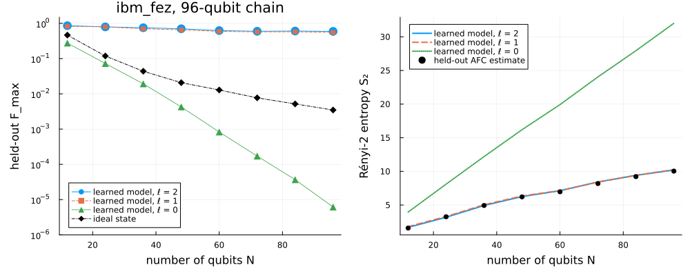
ผลลัพธ์ยืนยันทั้งสองข้อกล่าวอ้างของเปเปอร์บนโปรเซสเซอร์คนละตัว:
-
โมเดลอธิบายข้อมูลได้ดีกว่าสถานะอุดมคติมาก ที่ ค่า บนข้อมูล held-out ของโมเดล คือ 0.59 ± 0.10 เทียบกับ 0.0035 ของสถานะอุดมคติ เปเปอร์รายงานประมาณ 0.75 บน
ibm_brisbane -
เอนโทรปีของโมเดลสอดคล้องกับข้อมูลทดสอบที่ทุกค่า ที่ ได้ 10.2 จากโมเดลและ 10.0 ± 0.3 จากข้อมูลทดสอบ หรือ เทียบกับ 0.14 ถึง 0.15 บน
ibm_brisbaneรุ่นเก่ากว่า
การเปรียบเทียบขนาดหน้าต่างแสดงให้เห็นว่าข้อมูลอยู่ที่ไหน เมื่อ โมเดลดีเกือบเท่ากัน () ดังนั้นสำหรับข้อมูลชุดนี้ สหสัมพันธ์ที่ไกลกว่าไม่กี่ qubit เพิ่มอะไรได้น้อย เมื่อ product state พลาดการพันกันระหว่าง qubit ข้างเคียง เอนโทรปีของมันโตถึง 32 แทนที่จะเป็น 10 และ ของมันลดลงเร็วกว่าของสถานะอุดมคติด้วยซ้ำ เหลือ ที่
โปรดจำข้อจำกัดต่อไปนี้ไว้เมื่ออ่านตัวเลขเหล่านี้:
-
การแบ่งชุดฝึก แถบความคลาดเคลื่อนครอบคลุมเฉพาะความคลาดเคลื่อนทางสถิติของข้อมูลทดสอบ การแบ่งแบบสุ่มอื่น ๆ ของการตั้งค่าชุดเดียวกันให้ ระหว่าง 0.49 ถึง 0.59 ที่ สำหรับ
-
sweep สุดท้าย ตัวเรียนรู้คืนโมเดลจาก sweep สุดท้ายเสมอ ดังนั้นข้อมูลทดสอบจึงไม่เคยมีอิทธิพลต่อโมเดล
-
ความเป็นบวก โมเดลไม่ได้ถูกบังคับให้เป็น positive semidefinite ค่าลักษณะเฉพาะที่ติดลบที่สุดในหน้าต่างการเรียนรู้อยู่ที่ประมาณ ดังนั้น และ ของมันจึงอธิบายตัวดำเนินการ ไม่ใช่คุณสมบัติที่รับรองแล้วของสถานะทางกายภาพ
-
การแยกตัวประกอบ ทุกการประมาณค่า held-out อาศัยสมมติฐาน AFC ซึ่งการวัดเองไม่สามารถรับรองได้
ขั้นตอนถัดไป
-
ทำการทดลองซ้ำที่ความลึกสองด้วยพารามิเตอร์ของเปเปอร์สำหรับความลึกนั้น ( และ bond dimension สูงสุด 8) และหาว่าตัวเรียนรู้ต้องการการตั้งค่าการวัดกี่ชุด
-
เรียนรู้ด้วยการอัปเดตแบบสองไซต์แทน (
update=:two_siteในtraining_marginalsและlearn_mpo) ซึ่งตัด bond dimension ทิ้งหลังทุกขั้น และดูว่ามันทำงานอย่างไรเมื่อมีการตั้งค่าสำหรับฝึกน้อยลง -
เรียนรู้โดยไม่มี CRM prior (
prior=nothing) และเปรียบเทียบ fidelity บนข้อมูล held-out -
ใช้การวิเคราะห์เดียวกันกับการวัดบน
ibm_brisbaneที่ผู้เขียนเผยแพร่ -
อ่านภาคผนวกของเปเปอร์เพื่อดูที่มาของการอัปเดตและตัวประมาณค่า AFC
-
สำรวจโปรโตคอลการวัดแบบสุ่มอื่น ๆ ในตัวอย่างของ
RandomMeas.jl
เอกสารอ้างอิง
-
M. Votto, M. Ljubotina, C. Lancien, J. I. Cirac, P. Zoller, M. Serbyn, L. Piroli, and B. Vermersch, "Learning mixed quantum states in large-scale experiments", Phys. Rev. Lett. 136, 090801 (2026). arXiv:2507.12550
-
A. Elben, S. T. Flammia, H.-Y. Huang, R. Kueng, J. Preskill, B. Vermersch, and P. Zoller, "The randomized measurement toolbox", Nat. Rev. Phys. 5, 9 (2023). arXiv:2203.11374
-
H.-Y. Huang, R. Kueng, and J. Preskill, "Predicting many properties of a quantum system from very few measurements", Nat. Phys. 16, 1050 (2020). arXiv:2002.08953
-
A. Elben and B. Vermersch, "RandomMeas.jl: A Julia package for randomized measurements in quantum devices", Quantum 10, 2086 (2026). arXiv:2509.12749
-
B. Vermersch, A. Rath, B. Sundar, C. Branciard, J. Preskill, and A. Elben, "Enhanced estimation of quantum properties with common randomized measurements", PRX Quantum 5, 010352 (2024). arXiv:2304.12292
-
H. Zou, "Randomized measurements of a 96-qubit kicked-Ising state on ibm_fez", Zenodo (2026). doi:10.5281/zenodo.24116174