การเริ่มต้นของ ergodicity ข้ามสเกล
notebook นี้พาทำตามวิธีรันและวิเคราะห์การทดลองใน Onset of Ergodicity Across Scales on a Digital Quantum Processor [arXiv:2603.12236] ตั้งแต่โมเดลไปสู่ circuit, จาก bitstring ไปสู่ entropy, จากข้อมูลที่มีสัญญาณรบกวนไปสู่ผลลัพธ์ที่ลดข้อผิดพลาดแล้ว และจากการจำลอง 16 qubit ไปสู่การรัน 64 qubit บนโปรเซสเซอร์ IBM Quantum® Nighthawk โค้ดทั้งหมดอยู่ที่นี่ และแต่ละฟังก์ชันถูกนิยามตรงที่ต้องใช้เป็นครั้งแรก
| เวลา | หัวข้อ |
|---|---|
| 0–1 นาที | การตั้งค่า |
| 1–6 นาที | 1. จากโมเดลสู่ circuit |
| 6–12 นาที | 2. วัดอะไรและประมาณค่าอย่างไร |
| 12–19 นาที | 3. สัญญาณรบกวน และวิธีเอาออก |
| 19–24 นาที | 4. รันในระดับใหญ่ |
| 24–33 นาที | 5. ข้อมูลจากฮาร์ดแวร์ |
| 33–35 นาที | สรุป |
ทำตามไปด้วย รันเซลล์จากบนลงล่าง ไม่ต้องมีบัญชี IBM Quantum เซลล์ที่ส่ง hardware job ถูกปิดไว้ และหัวข้อ 5 วิเคราะห์การรันบนฮาร์ดแวร์ที่บันทึกไว้ ซึ่งเซลล์ตั้งค่าจะดาวน์โหลดไปที่ data/ คำถามสำหรับอภิปรายมีเครื่องหมาย Question ลองตอบก่อนเปิดดูคำตอบ
การตั้งค่า
ต้องใช้ Python 3.12 ขึ้นไปและแพ็กเกจต่อไปนี้
-
Qiskit SDK v2.5 ขึ้นไป พร้อมการรองรับ visualization
-
Qiskit Runtime v0.49 ขึ้นไป (
pip install qiskit-ibm-runtime) -
Qiskit Aer v0.17 ขึ้นไป (
pip install qiskit-aer) -
Samplomatic v0.21 ขึ้นไป (
pip install samplomatic) -
NumPy และ Matplotlib
เซลล์ตั้งค่ายังดาวน์โหลดการรันบนฮาร์ดแวร์ที่บันทึกไว้และ MPS reference (ราว 9 MB) ไปที่ data/ เว้นแต่ว่ามีอยู่แล้ว
# Added by doQumentation — installs the packages this notebook needs if they are missing
import importlib.util

_needed = {"matplotlib": "matplotlib", "numpy": "numpy", "qiskit": "qiskit", "qiskit_aer": "qiskit-aer", "qiskit_ibm_runtime": "qiskit-ibm-runtime", "samplomatic": "samplomatic"}
_missing = [pip for module, pip in _needed.items()
            if importlib.util.find_spec(module) is None]
# One at a time, so a package that fails to install does not block the others
for _pip in _missing:
    %pip install -q {_pip}
if not _missing:
    print("\u2713 All required packages are installed")
from math import comb
from pathlib import Path
from urllib.request import urlretrieve

import matplotlib.pyplot as plt
import numpy as np
from qiskit import ClassicalRegister, QuantumCircuit, QuantumRegister
from qiskit.primitives import StatevectorSampler
from qiskit.quantum_info import (
    PauliLindbladMap,
    QubitSparsePauli,
    Statevector,
)
from qiskit.transpiler import generate_preset_pass_manager
from qiskit_aer import AerSimulator
from qiskit_aer.noise import NoiseModel, ReadoutError, depolarizing_error
from qiskit_aer.primitives import SamplerV2 as AerSampler

RUN_ON_HARDWARE = (
    False  # True submits the 8x8 jobs in section 4 (needs Nighthawk access)
)
COMPUTE_MPS_REFERENCES = False  # True recomputes the MPS references in section 5 (about 18 minutes)

# Download the saved hardware run and MPS references, unless they are already in data/
data_url = "https://raw.githubusercontent.com/Qiskit/documentation/main/datasets/tutorials/onset-of-ergodicity"
Path("data").mkdir(exist_ok=True)
for name in ("hardware_run.npz", "mps_references_all.npz"):
    if not Path("data", name).exists():
        urlretrieve(f"{data_url}/{name}", Path("data", name))
1. จากโมเดลสู่ circuit
two-qubit gate
ทุก bond ของ lattice ได้ two-qubit gate แบบเดียวกัน ประกอบด้วย Heisenberg entangler ตามด้วยสนามสุ่ม:
โดย สุ่มอย่างสม่ำเสมอจาก สำหรับทุก gate
Question. คุณจะแยก เป็น gate ที่ฮาร์ดแวร์รันได้อย่างไร
คำตอบ
สนาม ง่าย คือการหมุน single-qubit บนแต่ละ qubit
entangler คือส่วนที่ยาก , และ สับเปลี่ยนกัน จึงแยกตัวประกอบเป็นการหมุนสามแบบ คือ , และ แต่ละแบบใช้ CNOT สองตัว รวมเป็นหกตัวต่อ gate
มีวิธีที่ดีกว่า gate สอง qubit ใด ๆ สร้างได้จาก CNOT อย่างมากสามตัวและการหมุน single-qubit circuit ที่เหมาะสมที่สุดเริ่มจากรูป และ entangler นี้มีรูปนั้นอยู่แล้วโดย จึงแมปตรงไปที่ CNOT สามตัว และมุมของ single-qubit เป็นเชิงเส้นใน โค้ดของการทดลองสร้าง gate ด้วยวิธีนี้
บนฮาร์ดแวร์ two-qubit gate ทุกตัวเพิ่มสัญญาณรบกวน ดังนั้นการลดจำนวน CNOT ลงครึ่งหนึ่งจึงสำคัญ
def xxyyzz_gate(circuit, coupling, i, j):
    # exp(iJ(XX + YY + ZZ)) with three CNOTs; only the rotation angles depend on J
    circuit.rz(-np.pi / 2, j)
    circuit.cx(j, i)
    circuit.rz(np.pi / 2 - 2 * coupling, i)
    circuit.ry(2 * coupling - np.pi / 2, j)
    circuit.cx(i, j)
    circuit.ry(np.pi / 2 - 2 * coupling, j)
    circuit.cx(j, i)
    circuit.rz(np.pi / 2, i)

def heisenberg_gate(circuit, coupling, i, j, h_i, h_j):
    # The entangler first, then the random fields exp(i h Z)
    xxyyzz_gate(circuit, coupling, i, j)
    circuit.rz(-2 * h_i, i)
    circuit.rz(-2 * h_j, j)

h_i, h_j = 0.3, -0.7
gate = QuantumCircuit(2)
heisenberg_gate(gate, 0.05 * np.pi, 0, 1, h_i, h_j)
gate.draw("mpl")

brickwork และ Floquet cycle
gate ปูเต็ม square lattice ใน sublayer สี่ชั้นของ bond ที่ไม่ซ้อนทับกัน เป็น brickwork คือ bond แนวนอนที่เริ่มจากคอลัมน์คู่ แล้วคอลัมน์คี่ แล้ว bond แนวตั้งที่เริ่มจากแถวคู่ แล้วแถวคี่ qubit อยู่ที่ตำแหน่ง
def brickwork_layers(num_cols, num_rows):
    # Bonds of the square lattice, in the four sublayers of the brickwork
    def qubit(x, y):
        return y * num_cols + x

    layers = []
    for p in (0, 1):  # horizontal bonds starting on even, then odd, columns
        layers.append(
            [
                (qubit(x, y), qubit(x + 1, y))
                for y in range(num_rows)
                for x in range(p, num_cols - 1, 2)
            ]
        )
    for p in (0, 1):  # vertical bonds starting on even, then odd, rows
        layers.append(
            [
                (qubit(x, y), qubit(x, y + 1))
                for y in range(p, num_rows - 1, 2)
                for x in range(num_cols)
            ]
        )
    return layers

brickwork_layers(4, 4)
[[(0, 1), (2, 3), (4, 5), (6, 7), (8, 9), (10, 11), (12, 13), (14, 15)],
 [(1, 2), (5, 6), (9, 10), (13, 14)],
 [(0, 4), (1, 5), (2, 6), (3, 7), (8, 12), (9, 13), (10, 14), (11, 15)],
 [(4, 8), (5, 9), (6, 10), (7, 11)]]
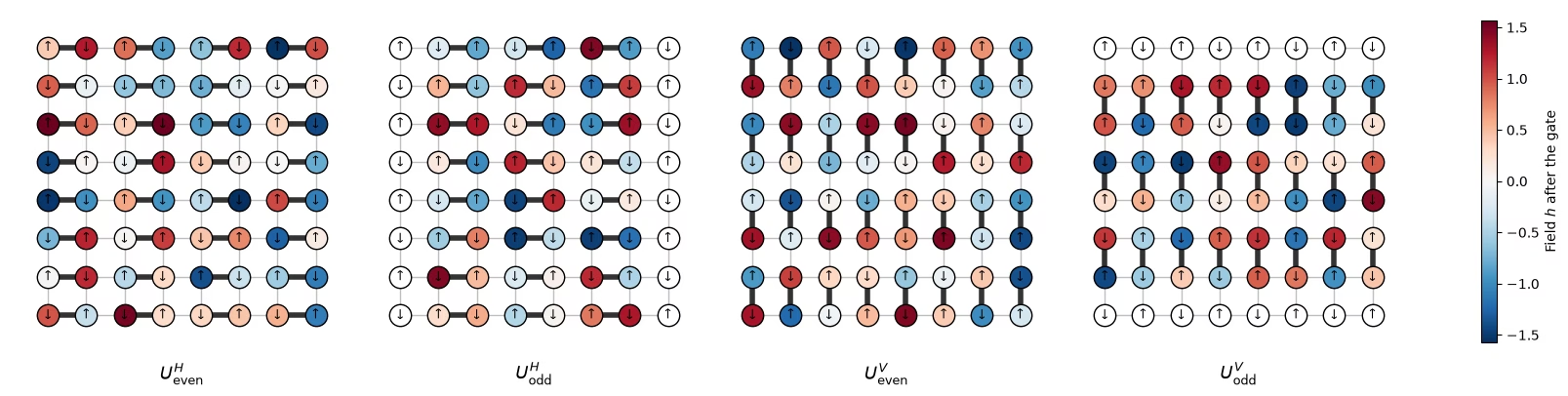
สี่ sublayer ประกอบเป็น Floquet cycle หนึ่งรอบ cycle ซ้ำ ครั้งด้วย สนามเดียวกัน ไดนามิกส์จึงสุ่มในเชิงพื้นที่และเป็นคาบในเชิงเวลา circuit เริ่มจากสถานะ Néel และ เท่ากับครึ่งหนึ่งของความยาวด้านของ lattice เซลล์ถัดไปวาด Floquet cycle หนึ่งรอบของ lattice ฮาร์ดแวร์ ทีละ sublayer ด้วยสนามจากการรันบนฮาร์ดแวร์ ในสไตล์ของ Figure 5 ในเปเปอร์ bond หนาคือ gate ของแต่ละ sublayer qubit แต่ละตัวที่ gate กระทำจะถูกลงสีตามสนามสุ่ม ที่มันได้รับต่อมา และ qubit ที่ว่างเป็นสีขาว ลูกศรแสดงสถานะเริ่มต้น Néel โดย แทน รูปในเปเปอร์ใช้ sublayer แนวตั้งก่อน ทั้งสองลำดับไม่คาดว่าจะเปลี่ยนฟิสิกส์
# circuit structure, 8x8 system:
side = 8
all_bonds = [bond for layer in brickwork_layers(side, side) for bond in layer]

# get the disorder parameters for a given system:
def sample_disorder(num_cols, num_rows, rng):
    # One pair of fields (h_i, h_j) per gate, reused in every Floquet cycle
    return [
        [
            (bond, tuple(rng.uniform(-np.pi / 2, np.pi / 2, 2)))
            for bond in layer
        ]
        for layer in brickwork_layers(num_cols, num_rows)
    ]

# build the structure for the 8x8 system
example_disorder = sample_disorder(
    side, side, np.random.default_rng(7)
)  # the hardware fields (section 4)
titles = [
    r"$U^H_\mathrm{even}$",
    r"$U^H_\mathrm{odd}$",
    r"$U^V_\mathrm{even}$",
    r"$U^V_\mathrm{odd}$",
]
norm = plt.Normalize(-np.pi / 2, np.pi / 2)
cmap = plt.get_cmap("RdBu_r")

fig, axes = plt.subplots(1, 4, figsize=(16, 4.8), layout="constrained")
for ax, title, sublayer in zip(axes, titles, example_disorder):
    for i, j in all_bonds:
        ax.plot(
            [i % side, j % side],
            [i // side, j // side],
            color="0.75",
            lw=1,
            zorder=0,
        )
    fields = {}
    for (i, j), (h_i, h_j) in sublayer:
        ax.plot(
            [i % side, j % side],
            [i // side, j // side],
            color="0.2",
            lw=4,
            zorder=1,
        )
        fields[i], fields[j] = h_i, h_j
    for q in range(side * side):
        x, y = q % side, q // side
        ax.scatter(
            x,
            y,
            s=260,
            color=cmap(norm(fields[q])) if q in fields else "white",
            edgecolor="black",
            zorder=2,
        )
        ax.text(
            x,
            y,
            "↓" if (x + y) % 2 else "↑",
            ha="center",
            va="center",
            fontsize=9,
            zorder=3,
        )
    ax.set_aspect("equal")
    ax.set_xlim(-1, side)  # padding, so the panels read as separate steps
    ax.set_ylim(side, -1)
    ax.axis("off")
    ax.set_title(title, y=-0.1, fontsize=13)
fig.colorbar(
    plt.cm.ScalarMappable(norm=norm, cmap=cmap),
    ax=axes,
    shrink=0.7,
    label="Field $h$ after the gate",
)
plt.show()
นิยามสถานะเริ่มต้น
# initial state
def neel_state(circuit, num_cols, num_rows, layout):
    for y in range(num_rows):
        for x in range(num_cols):
            if (x + y) % 2 == 1:
                circuit.x(layout[y * num_cols + x])
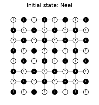
# The initial Néel state: |1⟩ (black, ↓) on odd sites, |0⟩ (white, ↑) on even sites

fig, ax = plt.subplots(figsize=(4, 4.4))
for i, j in all_bonds:
    ax.plot(
        [i % side, j % side],
        [i // side, j // side],
        color="0.75",
        lw=1,
        zorder=0,
    )
for q in range(side * side):
    x, y = q % side, q // side
    excited = (x + y) % 2 == 1
    ax.scatter(
        x,
        y,
        s=150,
        color="black" if excited else "white",
        edgecolor="black",
        zorder=2,
    )
    ax.text(
        x,
        y,
        "↓" if excited else "↑",
        ha="center",
        va="center",
        fontsize=7,
        color="white" if excited else "black",
        zorder=3,
    )
ax.set_aspect("equal")
ax.set_xlim(-1, side)
ax.set_ylim(side, -1)
ax.axis("off")
ax.set_title("Initial state: Néel", fontsize=13)
plt.show()
# actual circuit construction:
def heisenberg_floquet_circuit(
    num_cols, num_rows, coupling, num_cycles, disorder, measure=True
):
    num_qubits = num_cols * num_rows
    circuit = QuantumCircuit(num_qubits)
    neel_state(circuit, num_cols, num_rows, list(range(num_qubits)))
    cycle = QuantumCircuit(num_qubits)
    for sublayer in disorder:
        for (i, j), (h_i, h_j) in sublayer:
            heisenberg_gate(cycle, coupling, i, j, h_i, h_j)
    for _ in range(num_cycles):
        circuit.compose(cycle, inplace=True)
    if measure:
        circuit.measure_all()
    return circuit
ตัวอย่าง
การจำลองใช้ lattice สอง cycle และ coupling ที่ศึกษาในเปเปอร์ ใช้ชุดสนามเดียวซ้ำสำหรับทุก coupling
# simulation parameters:
num_cols = num_rows = 4
num_qubits = num_cols * num_rows
num_cycles = 2
couplings = (
    np.array([0.005, 0.01, 0.02, 0.03, 0.04, 0.05, 0.06, 0.08, 0.10, 0.125])
    * np.pi
)
disorder = sample_disorder(num_cols, num_rows, np.random.default_rng(42))

# circuit construction:
logical_circuits = [
    heisenberg_floquet_circuit(
        num_cols, num_rows, coupling, num_cycles, disorder
    )
    for coupling in couplings
]
logical_circuits[5].draw(output="mpl", fold=-1)

# transpiling the circuit:
pass_manager = generate_preset_pass_manager(
    optimization_level=3,
    basis_gates=["cz", "rz", "sx", "x"],
    seed_transpiler=7,
)
circuits = [pass_manager.run(circuit) for circuit in logical_circuits]

def two_qubit_stats(circuit):
    count = sum(1 for inst in circuit.data if inst.operation.num_qubits == 2)
    depth = circuit.depth(lambda inst: inst.operation.num_qubits == 2)
    return count, depth

stats = {two_qubit_stats(circuit) for circuit in circuits}
assert len(stats) == 1, "the CZ structure should not depend on J"
num_cz, depth = stats.pop()
print(
    f"{num_qubits} qubits: {num_cz} CZ gates in {depth} layers, for every coupling"
)
circuits[5].draw("mpl", fold=-1, scale=0.4)
16 qubits: 144 CZ gates in 24 layers, for every coupling

ไม่ต้องใช้คอมไพเลอร์ฉลาด ๆ เพราะ circuit (และการทดลอง) ถูกออกแบบมาสำหรับ IBM Nighthawk
จำลอง lattice
สำหรับ lattice คุณทำได้ทั้งสองอย่าง คือคำนวณสถานะที่แน่นอนที่ทุก coupling และสุ่มตัวอย่างทุก circuit ด้วย 10,000 shot เหมือนที่การทดลองทำ shot ถูกเก็บในรูปร่าง (batch, shot, qubit) ซึ่งเป็นเลย์เอาต์เดียวกับ randomization ในข้อมูลฮาร์ดแวร์ ในที่นี้ 10,000 shot ทั้งหมดเป็น batch เดียว ดังนั้น bootstrap ข้าม batch จึงไม่เพิ่มสัญญาณรบกวนจาก shot และแถบข้อผิดพลาดในกราฟถัดไปแสดงเพียงการกระจายระหว่างตำแหน่ง marginal
exact_states = [
    Statevector(
        heisenberg_floquet_circuit(
            num_cols, num_rows, c, num_cycles, disorder, measure=False
        )
    )
    for c in couplings
]

shots = 10_000
results = (
    StatevectorSampler(default_shots=shots, seed=1234).run(circuits).result()
)

# the output of the simulation for the 10 couplings
bits = [
    result.data.meas.to_bool_array(order="little").reshape(
        1, 10_000, num_qubits
    )
    for result in results
]

print(bits[0])
[[[False  True False ... False  True False]
  [False  True False ... False  True False]
  [False  True False ... False  True False]
  ...
  [False  True False ... False  True False]
  [False  True False ... False  True False]
  [False  True False ... False  True False]]]
2. วัดอะไรและประมาณค่าอย่างไร
IPR และ collision entropy
สำหรับ marginal ของ qubit ที่มีการแจกแจง bitstring ปริมาณที่ต้องประมาณคือ inverse participation ratio (IPR) ของการแจกแจง marginal และจากนั้นคือ collision entropy:
ยังเป็นความน่าจะเป็นที่สอง shot ตรงกันบน marginal สถานะผลคูณมี และสถานะสุ่มมี ดังนั้น จึงเพิ่มจาก 0 ไปถึงราว บิตเมื่อ marginal กลายเป็นสุ่ม
Estimator 1: นับคู่ของ shot
Question. คุณจะประมาณปริมาณนี้จาก shot ของคุณอย่างไร
คำตอบ
estimator แบบตรงไปตรงมาคำนวณแต่ละ จาก shot เป็น แล้วรวม estimator นี้มีความเอนเอียง
นับทุก shot ว่าตรงกับตัวเอง ซึ่งดันค่าประมาณให้สูงขึ้น โดยเฉลี่ยจะได้ แทนที่จะเป็น เนื่องจาก คือความน่าจะเป็นที่สอง shot ตรงกัน จึงให้นับเฉพาะคู่ของ shot ที่ ต่างกัน:
ค่านี้ไม่เอนเอียง และเป็นสิ่งที่ ipr_from_shots ด้านล่างคำนวณ
# IPR expectation values:

# refactor this function cause it does not scale
def ipr_from_shots(bits):
    # Pair-counting estimate of the IPR of a marginal: the fraction of pairs of different shots
    # that agree on it. bits holds the marginal's qubits only, with shape (randomizations, shots,
    # qubits), and all randomizations are pooled.
    n = bits.shape[-1]
    outcomes = bits @ 2 ** np.arange(
        n
    )  # each shot's marginal bitstring, read as an integer
    counts = np.bincount(outcomes.ravel())  # how often each outcome occurs
    total = counts.sum()
    return float((counts * (counts - 1)).sum() / (total * (total - 1)))

def collision_entropy(ipr):
    return -np.log2(ipr)
Estimator 2: การขยายแบบ Parseval
IPR เขียนได้อีกแบบผ่านพาริตี ของทุกเซตย่อย ที่ไม่ว่างของ marginal:
รูปแบบนี้สำคัญเพราะวิธี error mitigation เช่น PEA ทำงานกับค่าคาดหมาย ไม่ใช่กับความน่าจะเป็น หนึ่ง qubit: ความน่าจะเป็นของผลลัพธ์คือ และ ดังนั้น
marginal ขนาด : เมื่อกำหนดป้าย qubit เป็น marginal มี พาริตี คือ qubit เดี่ยว 4 ตัว, คู่ 6 คู่, สามตัว 4 ชุด และ marginal ทั้งหมด ดังนั้น
def parity_supports(patch):
    # All nonempty subsets S of the marginal
    return sorted(
        [
            tuple(q for k, q in enumerate(patch) if mask & (1 << k))
            for mask in range(1, 1 << len(patch))
        ],
        key=len,
    )

def parity_expectation_values(bits, supports):
    # Shot-averaged <Z_S> for every support, per randomization
    signs = 1 - 2 * bits.astype(np.int8)
    return np.stack(
        [signs[..., list(s)].prod(axis=-1).mean(axis=-1) for s in supports],
        axis=-1,
    )

# Example: the parities of a 3-qubit marginal made of lattice qubits 5, 6, and 9
print(parity_supports([5, 6, 9]))
print(f"A 3×3 marginal has {len(parity_supports(range(9)))} parities")
[(5,), (6,), (9,), (5, 6), (5, 9), (6, 9), (5, 6, 9)]
A 3×3 marginal has 511 parities
เฉลี่ยข้าม marginal
ฟังก์ชันที่มีประโยชน์เพิ่มเติม: ค่า Haar, การเลือก marginal, bootstrapping และการหาค่าเฉลี่ย
# functions for the Haar values on plots:
def haar_ipr(num_patch, num_qubits):
    # Mean IPR of a marginal for Haar-random states in the sector with num_qubits // 2 ones
    weight = num_qubits // 2
    dimension = comb(num_qubits, weight)
    total = 0
    for k in range(num_patch + 1):  # k ones on the marginal
        rest = (
            comb(num_qubits - num_patch, weight - k) if weight - k >= 0 else 0
        )
        total += comb(num_patch, k) * rest * (rest + 1)
    return total / (dimension * (dimension + 1))

def haar_entropy(num_patch, num_qubits):
    return collision_entropy(haar_ipr(num_patch, num_qubits))

# definitions of positions in the lattice:
def patch_qubits(anchor, shape, num_cols):
    # Lattice indices of a rectangular marginal with its top-left corner at anchor
    (x0, y0), (width, height) = anchor, shape
    return [
        (y0 + dy) * num_cols + (x0 + dx)
        for dy in range(height)
        for dx in range(width)
    ]

def all_positions(shape, num_cols, num_rows):
    # Every placement of a (width, height) marginal on the lattice
    width, height = shape
    return [
        patch_qubits((x, y), shape, num_cols)
        for y in range(num_rows - height + 1)
        for x in range(num_cols - width + 1)
    ]

# bootstrapping for error bars:
bootstrap_rng = np.random.default_rng(0)

def bootstrap_error(statistic, *samples, axis=0, num_resamples=50):
    # Shot noise of a statistic, from resampling the randomizations (along axis of every
    # sample) with replacement
    values = []
    for _ in range(num_resamples):
        resampled = [
            np.take(
                x,
                bootstrap_rng.integers(0, x.shape[axis], x.shape[axis]),
                axis=axis,
            )
            for x in samples
        ]
        values.append(statistic(*resampled))
    return float(np.std(values, ddof=1))

# averaging the ipr over marginals:
def average_ipr(iprs, shot_errors):
    # iprs and shot_errors have shape (positions, couplings). The mean IPR over positions, and its
    # error: the spread between positions plus the shot noise of each (law of total variance)
    iprs, shot_errors = np.asarray(iprs), np.asarray(shot_errors)
    count = len(iprs)
    variance = (
        iprs.var(axis=0, ddof=1) / count
        + (shot_errors**2).sum(axis=0) / count**2
    )
    return iprs.mean(axis=0), np.sqrt(variance)
# Calculating exact simulation entropies:
patch_shapes = {
    "1×1": (1, 1),
    "1×2": (2, 1),
    "2×2": (2, 2),
    "2×3": (3, 2),
    "3×3": (3, 3),
}

# calculate the exact entropies:
sim_positions = {
    label: all_positions(shape, num_cols, num_rows)
    for label, shape in patch_shapes.items()
}
exact_iprs = {  # shape (positions, couplings)
    label: np.array(
        [
            [(s.probabilities(qargs=q) ** 2).sum() for s in exact_states]
            for q in qubit_lists
        ]
    )
    for label, qubit_lists in sim_positions.items()
}
exact_entropies = {
    label: collision_entropy(v.mean(axis=0))
    for label, v in exact_iprs.items()
}

# Average IPR of every shape over its positions, from the sampled shots, then the entropy
iprs_from_shots = {}  # per shape: average IPR and its error, at every coupling
entropies_from_shots = {}  # per shape: average entropy and its error, at every coupling
for label, qubit_lists in sim_positions.items():
    iprs = [[ipr_from_shots(b[:, :, q]) for b in bits] for q in qubit_lists]

    # bootstrapping over subsampling for error bars:
    errors = [
        [bootstrap_error(ipr_from_shots, b[:, :, q]) for b in bits]
        for q in qubit_lists
    ]
    ipr, ipr_error = average_ipr(iprs, errors)
    iprs_from_shots[label] = (ipr, ipr_error)
    entropies_from_shots[label] = (
        collision_entropy(ipr),
        ipr_error / (ipr * np.log(2)),
    )
# Now plot the average IPR on the left, and the same averages as entropies on the right
colors = plt.cm.plasma(np.linspace(0.05, 0.8, len(patch_shapes)))
fig, (ax_ipr, ax_entropy) = plt.subplots(1, 2, figsize=(12.8, 4.2))
for (label, qubit_lists), color in zip(sim_positions.items(), colors):
    n = len(qubit_lists[0])
    ipr, ipr_error = iprs_from_shots[label]
    entropy, entropy_error = entropies_from_shots[label]
    # Left: the average IPR, with its exact value and its random-state value
    ax_ipr.axhline(haar_ipr(n, num_qubits), color=color, ls="dashdot", lw=0.9)
    ax_ipr.plot(
        couplings / np.pi, exact_iprs[label].mean(axis=0), color=color
    )
    ax_ipr.errorbar(
        couplings / np.pi,
        ipr,
        yerr=ipr_error,
        fmt="o",
        color=color,
        mec="white",
        ms=7,
        capsize=3,
        label=f"{label} ({len(qubit_lists)} positions)",
    )
    # Right: the average collision entropy
    ax_entropy.axhline(
        haar_entropy(n, num_qubits), color=color, ls="dashdot", lw=0.9
    )
    ax_entropy.plot(couplings / np.pi, exact_entropies[label], color=color)
    ax_entropy.errorbar(
        couplings / np.pi,
        entropy,
        yerr=entropy_error,
        fmt="o",
        color=color,
        mec="white",
        ms=7,
        capsize=3,
        label=f"{label} ({len(qubit_lists)} positions)",
    )
ax_ipr.set_yscale("log")
ax_ipr.set_ylabel("Average IPR")
ax_entropy.set_ylabel("Average collision entropy (bits)")
for ax in (ax_ipr, ax_entropy):
    ax.set_xlabel("Coupling $J/\\pi$")
fig.suptitle("Exact (lines) and sampled (dots), 4×4 lattice, 2 cycles")
ax_entropy.legend(title="Marginal", loc="upper left")
fig.tight_layout()
plt.show()
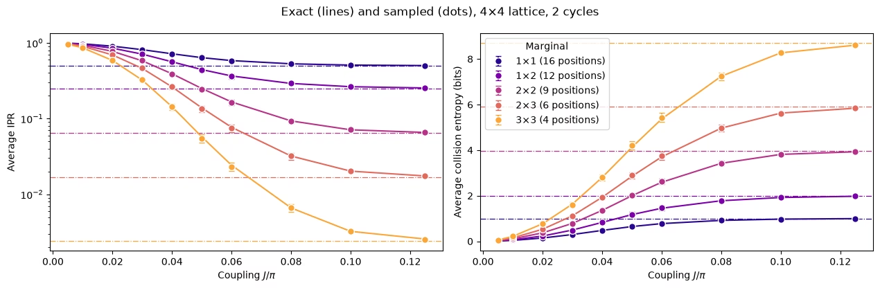
รูปร่างของ marginal ทุกแบบเพิ่มขึ้นอย่างราบรื่นไปสู่ค่าของสถานะสุ่ม และ marginal ที่ใหญ่กว่าจะไปถึงค่านั้นที่ ที่มากกว่า
3. Noise และวิธีแก้ไข
การจำลองที่มี noise
ทีนี้ลองเพิ่ม noise: depolarizing noise แบบสองคิวบิต 1% บน CZ gate ทุกตัว และ readout error 3% บนทุกคิวบิต โดยสุ่มตัวอย่างด้วย Qiskit Aer sampler วงจรนี้มี CZ gate 144 ตัว ซึ่งมี noise น้อยกว่าวงจรฮาร์ดแวร์ขนาด 8×8 มาก แต่ก็พอให้เห็นว่ามันส่งผลอย่างไร การจำลองใช้คัปปลิง 6 ค่า ค่าละ 4,000 shot และใช้เวลาประมาณ 1.5 นาที
คำถาม ก่อนรัน: noise จะทำให้ระบบดูเหมือน thermalize มากขึ้นหรือน้อยลง?
คำตอบ
มากขึ้น Noise ทำให้ผลลัพธ์ปนเปกันไปหมด ซึ่งดันการแจกแจง marginal ทุกตัวเข้าหาการแจกแจงสม่ำเสมอ ดังนั้น IPR ดิบจึงลดลงและเอนโทรปีเพิ่มขึ้น หากไม่ทำ mitigation noise จะดูเหมือน thermalization ที่ไม่ได้เกิดขึ้นจริง และจุด crossover จะออกมาเร็วเกินไป
# define the noise model

noise_model = NoiseModel()
# two qubit depolarizing noise:
noise_model.add_all_qubit_quantum_error(depolarizing_error(0.01, 2), ["cz"])
# symmetric readout noise:
noise_model.add_all_qubit_readout_error(
    ReadoutError([[0.97, 0.03], [0.03, 0.97]])
)

# simulation is done using trajectories
noisy_sampler = AerSampler(
    default_shots=4000,
    seed=1,
    options={"backend_options": {"noise_model": noise_model}},
)

# choose a subset of J values for speed:
noisy_indices = [
    0,
    2,
    3,
    5,
    7,
    9,
]  # J/π = 0.005, 0.02, 0.03, 0.05, 0.08, 0.125
noisy_results = noisy_sampler.run(
    [circuits[k] for k in noisy_indices]
).result()

# No twirling here, so the 20 "randomizations" are just batches of 200 shots
noisy_bits = {
    k: result.data.meas.to_bool_array(order="little").reshape(
        20, 200, num_qubits
    )
    for k, result in zip(noisy_indices, noisy_results)
}
# Calculating noisy entropies

# Average IPR of every shape over its positions, from the noisy shots, then the entropy
noisy_iprs = {}  # per shape: average IPR and its error, at every noisy coupling
noisy_entropies = {}  # per shape: average entropy and its error, at every noisy coupling
for label, qubit_lists in sim_positions.items():
    iprs = [
        [ipr_from_shots(noisy_bits[k][:, :, q]) for k in noisy_indices]
        for q in qubit_lists
    ]

    # bootstrapping over subsampling for error bars:
    errors = [
        [
            bootstrap_error(ipr_from_shots, noisy_bits[k][:, :, q])
            for k in noisy_indices
        ]
        for q in qubit_lists
    ]
    ipr, ipr_error = average_ipr(iprs, errors)
    noisy_iprs[label] = (ipr, ipr_error)
    noisy_entropies[label] = (
        collision_entropy(ipr),
        ipr_error / (ipr * np.log(2)),
    )
fig, (ax_ipr, ax_entropy) = plt.subplots(1, 2, figsize=(12.8, 4.2))
for (label, qubit_lists), color in zip(sim_positions.items(), colors):
    n = len(qubit_lists[0])
    ipr, ipr_error = noisy_iprs[label]
    entropy, entropy_error = noisy_entropies[label]
    # Left: the average IPR, with its exact value and its random-state value
    ax_ipr.axhline(haar_ipr(n, num_qubits), color=color, ls="dashdot", lw=0.9)
    ax_ipr.plot(
        couplings / np.pi, exact_iprs[label].mean(axis=0), color=color
    )
    ax_ipr.errorbar(
        couplings[noisy_indices] / np.pi,
        ipr,
        yerr=ipr_error,
        fmt="o",
        color=color,
        mec="white",
        ms=7,
        capsize=3,
        label=label,
    )
    # Right: the same averages as entropies
    ax_entropy.axhline(
        haar_entropy(n, num_qubits), color=color, ls="dashdot", lw=0.9
    )
    ax_entropy.plot(couplings / np.pi, exact_entropies[label], color=color)
    ax_entropy.errorbar(
        couplings[noisy_indices] / np.pi,
        entropy,
        yerr=entropy_error,
        fmt="o",
        color=color,
        mec="white",
        ms=7,
        capsize=3,
        label=label,
    )
ax_ipr.set_yscale("log")
ax_ipr.set_ylabel("Average IPR")
ax_entropy.set_ylabel("Average collision entropy (bits)")
for ax in (ax_ipr, ax_entropy):
    ax.set_xlabel("Coupling $J/\\pi$")
fig.suptitle("Exact (lines) and noisy raw estimates (dots)")
ax_entropy.legend(title="Marginal", loc="lower right")
fig.tight_layout()
plt.show()
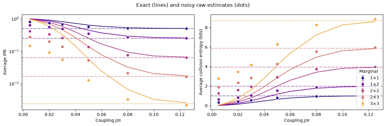
ลองคิดดู: คุณจะแก้ไขสิ่งนี้อย่างไร?
แนวทางที่แนะนำ
ที่ ค่าน้อย สถานะแทบไม่มี entanglement ดังนั้นคำตอบในอุดมคติตรงนั้นจึงคำนวณแบบคลาสสิกได้ไม่แพง แม้จะมี 64 คิวบิตก็ตาม นั่นแนะนำให้วัดผลของ noise ที่คัปปลิงสำหรับสอบเทียบค่าน้อย แล้วใช้ค่านั้นแก้ไขคัปปลิงอื่นทั้งหมด มีสองวิธีที่เป็นธรรมชาติ เรียกว่า low-entanglement calibration (LEC):
LEC บน IPR ปรับสเกลส่วนที่ IPR เกินค่าของการแจกแจงสม่ำเสมอ ด้วยตัวคูณหนึ่งตัวต่อ marginal:
LEC บนค่าคาดหวัง ปรับสเกล parity ทุกตัวของ marginal ด้วยตัวคูณของมันเอง แล้วสร้าง IPR ขึ้นใหม่ด้วยสูตร Parseval:
ในโค้ด parity ที่ปรับสเกลแล้วยกกำลังสองแต่ละตัวจะถูกลดอคติด้วยการลบความแปรปรวนของมัน เหมือนในหัวข้อที่ 2
ทั้งสองวิธีให้ผลเหมือนกันถ้า ทุกตัวเท่ากับ
Question. What are the pros and cons of these methods?
คำตอบ
Pros
-
ราคาถูก: ไม่ต้องใช้ข้อมูลเพิ่มจากอุปกรณ์ ใช้เพียงการจำลองแบบคลาสสิกที่
-
ใช้โครงสร้างของวงจร: ความลึกของวงจรและเลเยอร์ CZ ไม่เปลี่ยนตาม ดังนั้น noise ที่ จึงเป็น noise เดียวกับที่ อื่นทุกค่า
Cons
- สมมติว่าผลของ noise ต่อ observable ไม่ขึ้นกับ : ตัว noise เหมือนเดิม แต่วิธีที่มันลดทอน IPR หรือ แต่ละตัวอาจเปลี่ยนไปเมื่อ เพิ่มขึ้น
ทั้งสองวิธีกับการจำลองที่มี noise
# function to mitigate the IPR signal:
def mitigate_ipr_w_lec(
    ipr_raw, ipr_raw_calibration, ipr_ideal_calibration, num_patch
):
    # LEC on the IPR: one factor R0 for the excess over the uniform value
    uniform = 2.0**-num_patch
    factor = (ipr_ideal_calibration - uniform) / (
        ipr_raw_calibration - uniform
    )
    return uniform + factor * (ipr_raw - uniform)

# function used to calculate the target <Z> expectation values
def parities_from_probabilities(probabilities):
    # Ideal <Z_S> from a marginal distribution, in parity_supports order: subsets
    # by size, and in bitmask order within each size
    outcomes = np.arange(len(probabilities))
    masks = np.array(sorted(range(1, len(probabilities)), key=int.bit_count))
    signs = (-1.0) ** np.bitwise_count(outcomes[:, None] & masks[None, :])
    return np.asarray(probabilities) @ signs

# calculate boosting factors:
def lec_z_factors(calibration_parities, ideal_parities):
    # LEC on <Z>: one factor r_S per parity, from data with shape (randomizations, supports).
    return ideal_parities / calibration_parities.mean(axis=0)

# function to mitigate the IPR from <Z> expectation values:
def mitigate_ipr_w_lec_on_parities(
    parities, calibration_parities, ideal_calibration_parities, num_patch
):
    # LEC on <Z>: rescale each parity by its factor r_S = ideal / raw at J0, then rebuild the IPR
    # with Parseval. parities and calibration_parities have shape (randomizations, supports).
    # Each squared, rescaled parity is debiased by subtracting its variance, which to first
    # order combines the shot noise at J. The shot noise of r_S from J0 is omitted; including it
    # does not change the results.
    factors = lec_z_factors(calibration_parities, ideal_calibration_parities)
    mean = parities.mean(axis=0)  # mean over the twirling instances
    variance = parities.var(axis=0, ddof=1) / len(
        parities
    )  # variance of the mean
    rescaled = factors * mean
    rescaled_variance = factors**2 * variance
    return float((1 + np.sum(rescaled**2 - rescaled_variance)) / 2**num_patch)
def lec_estimates(patch_bits, parities, ideal, calibration, num_patch):
    # LEC on the IPR and on <Z> for one marginal position, at every coupling: values and shot
    # noise. patch_bits (the bits of the marginal only) and parities are per coupling, with
    # randomizations first.
    q_ideal = (ideal**2).sum()
    ideal_parities = parities_from_probabilities(ideal)

    def ipr_statistic(b, c):
        return mitigate_ipr_w_lec(
            ipr_from_shots(b), ipr_from_shots(c), q_ideal, num_patch
        )

    def z_statistic(p, c):
        return mitigate_ipr_w_lec_on_parities(p, c, ideal_parities, num_patch)

    values = {"LEC on IPR": [], "LEC on ⟨Z⟩": []}
    errors = {"LEC on IPR": [], "LEC on ⟨Z⟩": []}
    for k in range(len(patch_bits)):
        if (
            k == calibration
        ):  # both match the ideal value at J0 by construction
            for method in values:
                values[method].append(q_ideal)
                errors[method].append(0.0)
            continue
        values["LEC on IPR"].append(
            ipr_statistic(patch_bits[k], patch_bits[calibration])
        )
        errors["LEC on IPR"].append(
            bootstrap_error(
                ipr_statistic, patch_bits[k], patch_bits[calibration]
            )
        )
        values["LEC on ⟨Z⟩"].append(
            z_statistic(parities[k], parities[calibration])
        )
        errors["LEC on ⟨Z⟩"].append(
            bootstrap_error(z_statistic, parities[k], parities[calibration])
        )
    return values, errors

# getting all the data:
calibration_index = 0  # index of J0 = 0.005π in noisy_indices
mitigated = {
    "LEC on IPR": {},
    "LEC on ⟨Z⟩": {},
}  # per shape: (values, errors), each (positions, couplings)
for label, qubit_lists in sim_positions.items():
    n = len(qubit_lists[0])
    per_position = []
    for qubits in qubit_lists:
        supports = parity_supports(qubits)
        parities = [
            parity_expectation_values(noisy_bits[k], supports)
            for k in noisy_indices
        ]
        patch_bits = [noisy_bits[k][:, :, qubits] for k in noisy_indices]
        ideal = exact_states[noisy_indices[calibration_index]].probabilities(
            qargs=qubits
        )
        per_position.append(
            lec_estimates(patch_bits, parities, ideal, calibration_index, n)
        )
    for method in mitigated:
        mitigated[method][label] = (
            [p[0][method] for p in per_position],
            [p[1][method] for p in per_position],
        )

# Average over positions, then the entropy, for both methods
mitigated_entropies = {
    method: {} for method in mitigated
}  # per method and shape: entropy and its error
for method, by_shape in mitigated.items():
    for label, (values, errors) in by_shape.items():
        ipr, ipr_error = average_ipr(values, errors)
        mitigated_entropies[method][label] = (
            collision_entropy(ipr),
            ipr_error / (ipr * np.log(2)),
        )  # log here comes from error propagation
# Plot the data mitigated with both methods:

fig, axes = plt.subplots(1, 2, figsize=(12.8, 4.2), sharey=True)
for ax, (method, by_shape) in zip(axes, mitigated_entropies.items()):
    for (label, qubit_lists), color in zip(sim_positions.items(), colors):
        entropy, error = by_shape[label]
        ax.axhline(
            haar_entropy(len(qubit_lists[0]), num_qubits),
            color=color,
            ls="dashdot",
            lw=0.9,
        )
        ax.plot(couplings / np.pi, exact_entropies[label], color=color)
        ax.errorbar(
            couplings[noisy_indices] / np.pi,
            entropy,
            yerr=error,
            fmt="o",
            color=color,
            mec="white",
            ms=7,
            capsize=3,
            label=label,
        )
    ax.set_title(f"{method} (lines: exact)")
    ax.set_xlabel("Coupling $J/\\pi$")
axes[0].set_ylabel("Average collision entropy (bits)")
axes[0].legend(title="Marginal", loc="lower right")
fig.tight_layout()
plt.show()

# add the noisy data here too
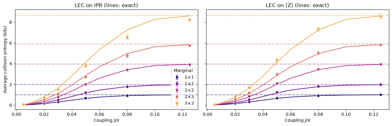
ทั้งสองวิธีกำจัดความเสียหายได้เกือบทั้งหมด: ค่าประมาณดิบในกราฟก่อนหน้าสุ่มเกินไปมาก ส่วนค่าที่ผ่าน mitigation แล้วตามเส้นโค้งที่แท้จริงได้ ความแตกต่างจะปรากฏที่ marginal ขนาดใหญ่
สำหรับ marginal ขนาดเล็ก ทั้งสองวิธีใช้ได้ผล สำหรับ marginal ขนาด LEC บน ใกล้เคียงกว่าอย่างชัดเจน
ทำไม LEC บน IPR จึงให้เอนโทรปีน้อยเกินไป เอนโทรปีน้อยเกินไปหมายความว่า IPR ใหญ่เกินไป: LEC บน IPR ขยายมันเกินจริง มันสมมติว่า noise ลดทอนการมีส่วนร่วมของ ทุกตัวต่อ IPR ด้วยตัวคูณเดียวกัน ที่ ทุกตัวใกล้ สตริงทั้งหมดจึงมีส่วนร่วมเท่ากัน และสตริงส่วนใหญ่มีน้ำหนักปานกลาง: จาก 511 สตริงของ marginal ขนาด มี 252 สตริงที่มีน้ำหนัก 4 หรือ 5 และมีเพียงเก้าสตริงที่มีน้ำหนัก 1 Noise ลดทอนสตริงมากขึ้นเมื่อน้ำหนักสูงขึ้น (readout error อย่างเดียวก็ลดทอนสตริงน้ำหนัก ด้วย ) ดังนั้นตัวคูณเดี่ยว จึงถูกกำหนดโดยการลดทอนของสตริงน้ำหนักปานกลางเป็นหลัก เมื่อ เพิ่มขึ้น ที่มีน้ำหนักสูงกว่าจะสลายเร็วที่สุด และ IPR จะถูกถ่ายทอดโดยสตริงน้ำหนักต่ำมากขึ้นเรื่อย ๆ ซึ่ง noise ลดทอนน้อยกว่า การขยายสตริงเหล่านี้ด้วยตัวคูณที่เรียนรู้จากสตริงที่ถูกลดทอนหนักกว่าเป็นหลักจึงทำให้ IPR ถูกขยายเกินจริง ผลนี้เพิ่มขึ้นตามขนาดของ marginal เพราะ marginal ที่ใหญ่กว่ามีช่วงน้ำหนักกว้างกว่า และมากที่สุดที่ ระดับกลาง หลังจากที่การผสมของสตริงเปลี่ยนไปแล้ว แต่ส่วนที่ IPR เกินค่าสม่ำเสมอยังมีความสำคัญอยู่
ทำไม LEC บน จึงผิดไปอีกทาง มันปรับสเกลแต่ละสตริงด้วยตัวคูณของมันเอง ดังนั้นการเลื่อนระหว่างน้ำหนักจึงไม่กระทบ มันสมมติเพียงว่าแต่ละสตริงยังคงการลดทอนแบบเดียวกับที่ เมื่อ เพิ่มขึ้น แต่ละตัวจะกระจายไปเป็นตัวดำเนินการที่มีน้ำหนักสูงขึ้น ซึ่งรับ noise มากกว่าที่ ตัวคูณจึงแก้ไขน้อยเกินไปเล็กน้อย และเอนโทรปีจึงออกมาสูงเกินไปเล็กน้อย
ดังนั้นการคาดการณ์ที่ต้องทดสอบบนฮาร์ดแวร์คือ: ยิ่ง marginal ใหญ่ LEC บน ยิ่งควรชนะ บนฮาร์ดแวร์ noise แรงกว่าและไม่ได้อยู่ในรูปแบบที่ทราบ
4. รันในระดับใหญ่
การทดลองบนฮาร์ดแวร์รันแลตทิซ ที่มีสี่รอบ: 64 คิวบิตและ CZ gate 1,344 ตัวใน 48 เลเยอร์ ที่คัปปลิงเก้าค่า มีห้าสิ่งที่เปลี่ยนไปเมื่อเทียบกับการจำลอง:
-
ต้องเรียนรู้ noise ซึ่งใช้ได้ก็ต่อเมื่อเลเยอร์ CZ คงที่
-
Twirling เปลี่ยน noise ของแต่ละเลเยอร์ให้เป็น Pauli channel ซึ่งเรียนรู้และขยายได้
-
Dynamical decoupling (DD) ปกป้องคิวบิตที่ว่างอยู่
-
การขยาย noise สำหรับ PEA รันในงานเดียวกับข้อมูลหลัก
-
การจำลอง MPS ที่ ค่าน้อยให้ค่าอ้างอิงแบบคลาสสิกสำหรับการลดข้อผิดพลาดแบบ LEC
เซลล์ที่ต้องใช้ backend จะรันก็ต่อเมื่อ RUN_ON_HARDWARE เป็น True การจำลอง MPS รันซ้ำได้โดยตั้ง COMPUTE_MPS_REFERENCES เป็น True เซลล์อื่นรันที่นี่
# hardware run parameters:
num_cols_hw = num_rows_hw = 8
num_qubits_hw = num_cols_hw * num_rows_hw
num_cycles_hw = 4
couplings_hw = (
    np.array([0.005, 0.01, 0.02, 0.03, 0.05, 0.07, 0.09, 0.11, 0.125]) * np.pi
)
calibration_hw = 0  # J0 = 0.005π
disorder_hw = sample_disorder(
    num_cols_hw, num_rows_hw, np.random.default_rng(7)
)

# if running PEA:
noise_factors = np.array([1.0, 1.5, 2.0])  # PEA noise-amplification factors
เลเยอร์ CZ คงที่
def compile_by_sublayer(
    num_cols,
    num_rows,
    coupling,
    num_cycles,
    disorder,
    pass_manager,
    layout=None,
    num_physical_qubits=None,
):
    # Compile each sublayer once and repeat it with barriers, so the CZ layers are the
    # same in every cycle and at every coupling. The registers are named explicitly
    # because register names enter Samplomatic's box hashes. Bits land in lattice order.
    num_qubits = num_cols * num_rows
    if layout is None:
        layout, num_physical_qubits = list(range(num_qubits)), num_qubits
    blocks = []
    for sublayer in disorder:
        block = QuantumCircuit(num_qubits)
        for (i, j), (h_i, h_j) in sublayer:
            heisenberg_gate(block, coupling, i, j, h_i, h_j)
        blocks.append(pass_manager.run(block))
    circuit = QuantumCircuit(
        QuantumRegister(num_physical_qubits, "q"),
        ClassicalRegister(num_qubits, "meas"),
    )
    neel_state(circuit, num_cols, num_rows, layout)
    for _ in range(num_cycles):
        for block in blocks:
            circuit.compose(block, inplace=True)
            circuit.barrier(layout)
    circuit.measure(layout, range(num_qubits))
    return circuit
Box สำหรับการเรียนรู้ noise
จากนั้น Samplomatic boxing pass manager จะจัดกลุ่มแต่ละวงจรเป็น box: หนึ่ง box ต่อหนึ่งเลเยอร์ CZ และอีกหนึ่ง box สำหรับการวัด แต่ละ box มีการอ้างอิงถึงโมเดล noise ที่ต้องใช้ คุณจึงตรวจสอบได้ว่าทุกคัปปลิงใช้ box ชุดเดียวกัน เซลล์ถัดไปทำเช่นนี้กับวงจร ของการรันบนฮาร์ดแวร์ ที่คอมไพล์เป็น CZ gate โดยไม่ใช้ backend และพิมพ์ box ที่การเรียนรู้ noise จะใช้หาลักษณะเฉพาะ
from samplomatic import build
from samplomatic.transpiler import generate_boxing_pass_manager
from samplomatic.utils import find_unique_box_instructions

boxing_pass_manager = generate_boxing_pass_manager(
    enable_gates=True,  # twirl the CZ layers
    enable_measures=True,  # twirl the measurements
    inject_noise_targets="gates",  # PEA amplifies the noise of the CZ layers only
    inject_noise_strategy="uniform_modification",
)

def noise_refs(boxed_circuit):
    return sorted(
        annotation.ref
        for box in find_unique_box_instructions(boxed_circuit.data)
        for annotation in box.operation.annotations
        if hasattr(annotation, "ref")
    )

# The 8x8 hardware circuits, compiled to CZ gates on the lattice qubits (no backend needed)
compiled_8x8 = [
    compile_by_sublayer(
        num_cols_hw, num_rows_hw, c, num_cycles_hw, disorder_hw, pass_manager
    )
    for c in couplings_hw
]
boxed_8x8 = [boxing_pass_manager.run(circuit) for circuit in compiled_8x8]
assert all(
    noise_refs(b) == noise_refs(boxed_8x8[0]) for b in boxed_8x8
), "layers differ between couplings"
num_cz, depth = two_qubit_stats(compiled_8x8[0])
print(
    f"{num_qubits_hw} qubits: {num_cz} CZ gates in {depth} layers, for every coupling"
)
for box in find_unique_box_instructions(boxed_8x8[0].data):
    ops = box.operation.blocks[0].count_ops()
    print(
        f"{box.operation.num_qubits}-qubit box: {ops.get('cz', 0)} CZ, {ops.get('measure', 0)} measurements"
    )
print(
    f"All {len(boxed_8x8)} couplings share these {len(find_unique_box_instructions(boxed_8x8[0].data))} boxes"
)
64 qubits: 1344 CZ gates in 48 layers, for every coupling
64-qubit box: 32 CZ, 0 measurements
64-qubit box: 24 CZ, 0 measurements
64-qubit box: 32 CZ, 0 measurements
64-qubit box: 24 CZ, 0 measurements
64-qubit box: 0 CZ, 64 measurements
All 9 couplings share these 5 boxes
ทำ twirl ให้วงจร
ในทุกการสุ่ม Samplomatic จะใส่ Pauli gate แบบสุ่มก่อนแต่ละ box และ gate ชดเชยหลัง box นั้น โดยรวมเข้ากับ single-qubit gate ข้างเคียง เมื่อเฉลี่ยตลอดการสุ่ม noise ของแต่ละเลเยอร์จะกลายเป็น Pauli channel ซึ่ง NoiseLearnerV3 เรียนรู้ได้ในรูปโมเดล sparse Pauli-Lindblad และขั้นตอน PEA ขยายได้ Measurement twirling จะสุ่มพลิกบิตก่อนการอ่านค่า การพลิกเหล่านั้นถูกยกเลิกด้วยซอฟต์แวร์ ซึ่งทำให้ readout noise สมมาตร และเป็นพื้นฐานของการแก้ readout (TREX)
เวิร์กโฟลว์บนฮาร์ดแวร์
เลือกคิวบิต คอมไพล์วงจร แล้วเรียนรู้ noise และรัน sweep เซลล์เหล่านี้ถูกปิดไว้ที่นี่
เลือกคิวบิต กริดสี่เหลี่ยมของ Nighthawk รองรับแลตทิซ ได้โดยไม่ต้องใช้ SWAP gate เซลล์นี้ให้คะแนนสี่เหลี่ยมผืนผ้า ทุกอันของกริดตาม CZ error และ readout error ที่รายงาน แล้วเลือกอันที่ดีที่สุด
def square_layouts(backend, side):
    # Every side x side rectangle of the square qubit grid that supports all bonds
    target = backend.target

    def has_cz(a, b):
        return (a, b) in target["cz"] or (b, a) in target["cz"]

    stride = next(
        s
        for s in (10, 12)
        if all(has_cz(q, q + s) for q in range(backend.num_qubits - s))
    )
    layouts = []
    for y0 in range(backend.num_qubits // stride - side + 1):
        for x0 in range(stride - side + 1):
            layout = [
                stride * (y0 + y) + x0 + x
                for y in range(side)
                for x in range(side)
            ]
            bonds = [
                bond
                for layer in brickwork_layers(side, side)
                for bond in layer
            ]
            if all(has_cz(layout[i], layout[j]) for i, j in bonds):
                layouts.append(((x0, y0), layout))
    return layouts

def layout_score(backend, layout, side, uses_per_bond):
    # Minus the summed log-fidelity of the bonds (each used uses_per_bond times) and readouts
    properties, target = backend.properties(), backend.target
    cz_errors = []
    for i, j in (
        bond for layer in brickwork_layers(side, side) for bond in layer
    ):
        pair = (
            (layout[i], layout[j])
            if (layout[i], layout[j]) in target["cz"]
            else (layout[j], layout[i])
        )
        cz_errors.append(properties.gate_error("cz", pair))
    readout_errors = [properties.readout_error(q) for q in layout]
    if max(cz_errors) >= 0.5 or max(readout_errors) >= 0.25:
        return np.inf  # an unusable qubit or bond
    return float(
        -uses_per_bond * np.log1p(-np.array(cz_errors)).sum()
        - np.log1p(-np.array(readout_errors)).sum()
    )

if RUN_ON_HARDWARE:
    from qiskit_ibm_runtime import QiskitRuntimeService

    def holds_lattice(backend):
        try:
            return bool(square_layouts(backend, num_cols_hw))
        except (KeyError, StopIteration):
            return False

    service = QiskitRuntimeService()
    candidates = [
        b
        for b in service.backends(operational=True, simulator=False)
        if holds_lattice(b)
    ]
    backend = min(candidates, key=lambda b: b.status().pending_jobs)
    score, origin, initial_layout = min(
        (
            layout_score(backend, layout, num_cols_hw, 3 * num_cycles_hw),
            origin,
            layout,
        )
        for origin, layout in square_layouts(backend, num_cols_hw)
    )
    print(f"{backend.name}: origin {origin}, score {score:.2f}")
คอมไพล์ ขั้นตอนเดียวกับข้างต้นบนคิวบิตที่เลือก ตามด้วย build ซึ่งเปลี่ยนแต่ละวงจรที่มี box ให้เป็นวงจรเทมเพลตและ samplex คือสูตรสำหรับสุ่ม twirling gate และ noise ที่ฉีดเข้าไป DD ถูกเพิ่มเข้าไปในเทมเพลต
if RUN_ON_HARDWARE:
    from qiskit_ibm_runtime.executor.dynamical_decoupling import (
        generate_dd_pass_manager,
    )
    from qiskit_ibm_runtime.options import DynamicalDecouplingOptions

    # PEA structure functions:
    target_pass_manager = generate_preset_pass_manager(
        target=backend.target,
        optimization_level=3,
        initial_layout=initial_layout,
        routing_method="none",
        seed_transpiler=7,
    )
    boxed_hw = [
        boxing_pass_manager.run(
            compile_by_sublayer(
                num_cols_hw,
                num_rows_hw,
                coupling,
                num_cycles_hw,
                disorder_hw,
                target_pass_manager,
                layout=initial_layout,
                num_physical_qubits=backend.num_qubits,
            )
        )
        for coupling in couplings_hw
    ]
    assert all(noise_refs(b) == noise_refs(boxed_hw[0]) for b in boxed_hw)
    unique_boxes_hw = find_unique_box_instructions(boxed_hw[0].data)

    # DD pass:
    dd_pass_manager = generate_dd_pass_manager(
        backend,
        DynamicalDecouplingOptions(
            enable=True,
            sequence_type="XY4",
            scheduling_method="alap",
            extra_slack_distribution="middle",
            skip_reset_qubits=False,
        ),
    )
    templates = []
    for circuit in boxed_hw:
        template, samplex = build(circuit)
        templates.append((dd_pass_manager.run(template), samplex))
เรียนรู้ noise และรัน sweep งาน NoiseLearnerV3 หนึ่งงานเรียนรู้ทั้งห้า box: โมเดล Pauli-Lindblad สำหรับแต่ละเลเยอร์ CZ ทั้งสี่ และ readout noise ของ box การวัด จากนั้น QuantumProgram หนึ่งตัวบรรจุคัปปลิงทั้งเก้าค่า แต่ละรายการได้เทมเพลต samplex โมเดล noise ที่เรียนรู้มา และสเกล noise สามค่า สเกล 0 คือข้อมูลที่ไม่ได้ขยายสำหรับทั้งสองวิธี LEC สเกล 0.5 และ 1 เพิ่ม noise ที่เรียนรู้มา 50% และ 100% สำหรับ PEA ซึ่ง extrapolate กลับไปที่ noise เป็นศูนย์ ขั้นตอนนี้ใช้เวลา QPU ประมาณ 40 วินาที
if RUN_ON_HARDWARE:
    from qiskit_ibm_runtime import Executor, NoiseLearnerV3, QuantumProgram

    # Learn the noise of the five boxes
    learner = NoiseLearnerV3(backend)
    learner.options.num_randomizations = 32
    learner.options.shots_per_randomization = 128
    # Up to 24 layer pairs, the depth of the 48-layer circuits
    learner.options.layer_pair_depths = [0, 1, 2, 4, 16, 24]
    learner_job = learner.run(unique_boxes_hw)
    print("Noise learning job:", learner_job.job_id())

    # Run the sweep, with the learned noise amplified by each of the noise factors
    noise_maps = learner_job.result().to_dict(
        instructions=unique_boxes_hw, require_refs=False
    )
    program = QuantumProgram(shots=200)
    for template, samplex in templates:
        program.append_samplex_item(
            template,
            samplex=samplex,
            samplex_arguments={
                "pauli_lindblad_maps": noise_maps,
                **{
                    f"noise_scales.{ref}": (noise_factors - 1).reshape(-1, 1)
                    for ref in noise_maps
                },
            },
            shape=(len(noise_factors), 200),  # noise scales x randomizations
        )
    executor_job = Executor(backend).run(program)
    print("Executor job:", executor_job.job_id())
    # Section 5 converts the results of these two jobs and saves them
5. ข้อมูลจากฮาร์ดแวร์
หัวข้อนี้สำรวจว่าวิธีการก่อนหน้านี้ทำงานได้ดีเพียงใดกับข้อมูลฮาร์ดแวร์จริงจากโปรเซสเซอร์ Nighthawk
โหลดการรัน
เมื่อตั้ง RUN_ON_HARDWARE เป็น True เซลล์ถัดไปจะแปลงผลลัพธ์ของสองงานจากหัวข้อที่ 4 และบันทึกลงใน data/hardware_run_new.npz ในรูปแบบเดียวกับการรันที่บันทึกไว้ เพื่อให้วิเคราะห์การรันใหม่ซ้ำได้ภายหลัง ไม่เช่นนั้นจะโหลดการรันที่บันทึกไว้จาก data/hardware_run.npz บิตถูกอัดไปตามแกนคิวบิตเพื่อประหยัดพื้นที่
ถ้า kernel รีสตาร์ตระหว่างที่งานกำลังรัน อย่าส่งงานซ้ำ ให้รันเซลล์ก่อนการเรียกสุดท้ายในหัวข้อที่ 4 ใหม่ ตรวจสอบว่าเลือกคิวบิตชุดเดียวกัน และตั้ง learner_job และ executor_job เป็น service.job(job_id) โดยใช้ job ID ที่พิมพ์ออกมาในหัวข้อที่ 4
if RUN_ON_HARDWARE:

    def unflip(item_result):
        # Undo the measurement twirling of an Executor item: flip back the bits that were flipped
        return item_result["meas"] ^ item_result["measurement_flips.meas"]

    learner_result = learner_job.result()
    raw_bits = [unflip(item) for item in executor_job.result()]

    # The learned readout map indexes the measured qubits in ascending physical order;
    # relabel it to lattice order
    measurement_box_index = next(
        k
        for k, box in enumerate(unique_boxes_hw)
        if "measure" in box.operation.blocks[0].count_ops()
    )
    measurement_box = next(
        inst
        for inst in boxed_hw[0].data
        if inst.operation.name == "box"
        and "measure" in inst.operation.blocks[0].count_ops()
    )
    measured = sorted(
        boxed_hw[0].find_bit(q).index for q in measurement_box.qubits
    )
    lattice_index = {physical: q for q, physical in enumerate(initial_layout)}
    readout_map = (
        learner_result[measurement_box_index]
        .to_pauli_lindblad_map()
        .apply_layout([lattice_index[p] for p in measured], num_qubits_hw)
    )

    # Save the run in the same format as the saved run, so it can be analyzed again later
    terms = readout_map.to_sparse_list()
    np.savez_compressed(
        "data/hardware_run_new.npz",
        bits=np.packbits(np.stack(raw_bits), axis=-1, bitorder="little"),
        labels=np.array([label for label, _, _ in terms]),
        indices=np.concatenate(
            [np.asarray(support) for _, support, _ in terms]
        ),
        rates=np.array([rate for _, _, rate in terms]),
        physical_qubits=np.array(initial_layout),
        couplings_over_pi=couplings_hw / np.pi,
        noise_factors=noise_factors,
    )
else:
    saved = np.load(
        "data/hardware_run.npz"
    )  # or data/hardware_run_new.npz, for a new run
    raw_bits = list(
        np.unpackbits(
            saved["bits"], axis=-1, count=num_qubits_hw, bitorder="little"
        ).astype(bool)
    )
    labels = [str(label) for label in saved["labels"]]
    indices = np.split(
        saved["indices"], np.cumsum([len(label) for label in labels])[:-1]
    )
    readout_map = PauliLindbladMap.from_sparse_list(
        list(zip(labels, indices, saved["rates"])), num_qubits_hw
    )

print(f"{len(raw_bits)} couplings, bits per coupling: {raw_bits[0].shape}")
print(
    f"Readout noise: {readout_map.num_terms} terms on {readout_map.num_qubits} qubits"
)
9 couplings, bits per coupling: (3, 200, 200, 64)
Readout noise: 64 terms on 64 qubits
ค่าอ้างอิงแบบคลาสสิก
ทั้งสองวิธี LEC ต้องการการแจกแจง marginal ในอุดมคติที่ และการทดสอบต้องใช้ค่าในอุดมคติที่คัปปลิงที่กันไว้ และ ค่าเหล่านี้มาจากการจำลอง matrix product state (MPS) ที่บันทึกไว้สำหรับทุกตำแหน่งที่วางรูปร่าง marginal แต่ละแบบบนแลตทิซ ตามในเปเปอร์ และสำหรับทุกบล็อก ที่ไม่ซ้อนกันที่ ที่ ค่าเหล่านี้ลู่เข้าที่ bond dimension ที่ และ ใช้ และที่ ค่ายังเปลี่ยนไปได้ถึงประมาณ 13% จาก สำหรับ marginal ขนาด ดังนั้นให้ถือว่าเป็นค่าประมาณตรงนั้น เซลล์ถัดไปคำนวณค่าเหล่านี้ถ้า COMPUTE_MPS_REFERENCES เป็น True ซึ่งใช้เวลาประมาณ 18 นาที ไม่เช่นนั้นจะโหลดผลลัพธ์ที่บันทึกไว้ ซึ่งจัดเก็บด้วยดัชนีคัปปลิง bond dimension และ marginal
# Every placement of every shape on the 8x8 lattice
positions = {
    label: all_positions(shape, num_cols_hw, num_rows_hw)
    for label, shape in patch_shapes.items()
}
reference_settings = [
    (calibration_hw, 32),
    (calibration_hw, 64),
    (1, 128),
    (2, 64),
    (2, 128),
]  # (coupling, χ)

if COMPUTE_MPS_REFERENCES:

    def mps_patch_probabilities(coupling, patches, bond_dimension):
        # Distributions of the given marginals after the 8x8 circuit, from an MPS simulation
        simulator = AerSimulator(
            method="matrix_product_state",
            matrix_product_state_max_bond_dimension=bond_dimension,
            matrix_product_state_truncation_threshold=1e-12,
        )
        circuit = heisenberg_floquet_circuit(
            num_cols_hw,
            num_rows_hw,
            coupling,
            num_cycles_hw,
            disorder_hw,
            measure=False,
        )
        circuit = generate_preset_pass_manager(
            optimization_level=1, basis_gates=["cx", "u"], seed_transpiler=7
        ).run(circuit)
        for label, qubits in patches.items():
            circuit.save_probabilities(qubits, label=label)
        data = simulator.run(circuit, shots=1).result().data(0)
        return {label: np.asarray(data[label]) for label in patches}

    placements = {
        f"{label} {k}": qubits
        for label, patch_list in positions.items()
        for k, qubits in enumerate(patch_list)
    }
    tiles = {
        f"site {q}": [q] for q in range(num_qubits_hw)
    } | {  # for the lattice map at J0
        f"block {x},{y}": patch_qubits((2 * x, 2 * y), (2, 2), num_cols_hw)
        for y in range(num_rows_hw // 2)
        for x in range(num_cols_hw // 2)
    }
    computed = {}
    for index, chi in reference_settings:
        targets = (
            placements | tiles
            if (index, chi) == (calibration_hw, 64)
            else placements
        )
        for key, p in mps_patch_probabilities(
            couplings_hw[index], targets, chi
        ).items():
            computed[f"{index}/{chi}/{key}"] = p
    np.savez_compressed("data/mps_references_all.npz", **computed)
    saved = computed
else:
    saved = np.load("data/mps_references_all.npz")

references = {}  # (coupling index, bond dimension) -> {marginal key: distribution}
for name in saved:
    index, chi, key = name.split("/", 2)
    references.setdefault((int(index), int(chi)), {})[key] = saved[name]
คุณภาพข้อมูล: coupler / คิวบิตที่ผิดปกติ
ก่อนอื่น ดูที่คัปปลิงต่ำสุด ซึ่งค่าคาดหวังควรใกล้เคียงกับลายกระดานหมากรุก Néel
# <Z> of every site at J0: the MPS reference, and the hardware data at noise factor 1
z_reference = np.array(
    [
        parities_from_probabilities(
            references[(calibration_hw, 64)][f"site {q}"]
        )[0]
        for q in range(num_qubits_hw)
    ]
)
z_measured = 1 - 2 * raw_bits[calibration_hw][0].mean(axis=(0, 1))
fig, axes = plt.subplots(1, 2, figsize=(11, 4.6), layout="constrained")
fig.get_layout_engine().set(wspace=0.12)  # white space between the two panels
edges = np.arange(num_cols_hw + 1) - 0.5
for ax, values, title in zip(
    axes, (z_reference, z_measured), ("MPS reference", "Hardware")
):
    mesh = ax.pcolormesh(
        edges,
        edges,
        values.reshape(num_rows_hw, num_cols_hw),
        cmap="RdBu_r",
        vmin=-1,
        vmax=1,
        edgecolors="white",
    )
    ax.set_aspect("equal")
    ax.invert_yaxis()
    ax.set_xticks([])
    ax.set_yticks([])
    ax.set_title(
        f"{title}, $J_0 = {couplings_hw[calibration_hw] / np.pi:g}\\pi$"
    )
fig.colorbar(
    mesh, ax=axes, shrink=0.8, label=r"$\langle Z \rangle$ of each site"
)
plt.show()

คำถาม เมื่อดูแผนที่ฮาร์ดแวร์ อะไรที่เด่นออกมา?
คำตอบ
ตำแหน่งสีซีด ซึ่งสูญเสียสัญญาณไปเกือบทั้งหมด ทั้งที่สถานะที่ ใกล้เคียงสถานะ Néel ตำแหน่งเหล่านี้สำคัญเพราะ LEC หารด้วยสัญญาณที่เหลืออยู่ที่ ไม่ว่าจะเหลือเท่าใด: คิวบิตที่แทบไม่มีสัญญาณจะให้ตัวคูณแก้ไขที่ใหญ่มากและมี noise และคิวบิตแบบนี้เพียงไม่กี่ตัวก็อาจครอบงำ marginal ทุกตัวที่มันอยู่ได้
กฎที่ใช้เฉพาะข้อมูล: คิวบิตถือว่าผิดปกติถ้า IPR คิวบิตเดี่ยวของมันที่ อยู่ภายใน ของ ซึ่งเป็นค่าของคิวบิตที่ผสมเต็มที่ เนื่องจาก IPR ของหนึ่งคิวบิตคือ กฎนี้จึงทำเครื่องหมายคิวบิตที่มี Marginal ที่มีตำแหน่งที่ถูกทำเครื่องหมายจะถูกตัดออกในส่วนต่อไป
site_iprs = np.array(
    [
        ipr_from_shots(raw_bits[calibration_hw][0][:, :, [q]])
        for q in range(num_qubits_hw)
    ]
)
# |IPR - 1/2| < 0.25**2 / 2 is the same as |<Z>| < 0.25
flagged = {
    q for q in range(num_qubits_hw) if abs(site_iprs[q] - 0.5) < 0.25**2 / 2
}
print(
    f"Median single-qubit IPR at J0: {np.median(site_iprs):.2f}; flagged lattice sites {sorted(flagged)}"
)
Median single-qubit IPR at J0: 0.77; flagged lattice sites [19, 24, 25, 27, 32]
เลือก marginal ที่จะนำมาเฉลี่ย
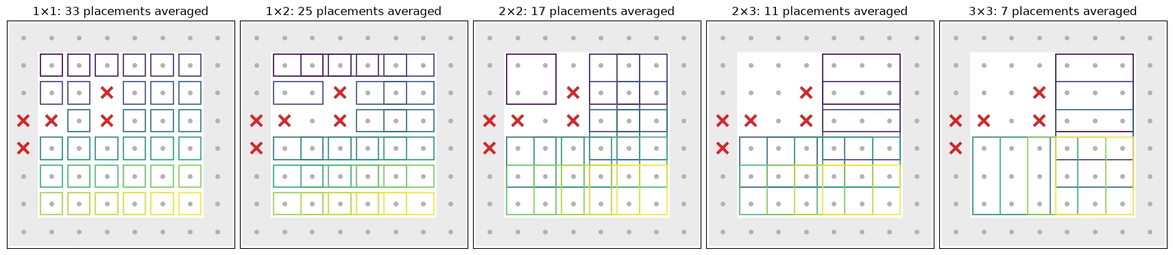
เซลล์ถัดไปแสดงว่าตำแหน่งวางของแต่ละรูปร่างใดบ้างที่เข้าไปอยู่ในค่าเฉลี่ยด้านล่าง: ทุกตำแหน่งในส่วนกลางของแลตทิซที่ไม่มีตำแหน่งที่ถูกทำเครื่องหมาย (กากบาทสีแดง) ตำแหน่งที่แตะขอบ (แรเงา) ถูกตัดออก คิวบิตขอบมีพันธะน้อยกว่า จึงสับเปลี่ยนช้ากว่า เมื่อเฉลี่ยแยกต่างหาก ค่าจะข้าม crossover ช้ากว่าตำแหน่งส่วนกลางเต็มหนึ่งขั้นของ สำหรับทุกรูปร่างและทุกวิธี ตำแหน่งที่นำมาเฉลี่ยแต่ละตำแหน่งมีกล่องของตัวเอง โดยมีสีตามตำแหน่ง
def touches_edge(qubits):
    # Whether a placement includes a site on the edge of the lattice
    return any(
        q % num_cols_hw in (0, num_cols_hw - 1)
        or q // num_cols_hw in (0, num_rows_hw - 1)
        for q in qubits
    )

# The placements of each shape that enter the averages: in the bulk, and without a flagged site
kept_placements = {
    label: [
        k
        for k, qubits in enumerate(patch_list)
        if not touches_edge(qubits) and not set(qubits) & flagged
    ]
    for label, patch_list in positions.items()
}
placement_cmap = plt.get_cmap("viridis")
fig, axes = plt.subplots(
    1, len(positions), figsize=(17, 4.4), layout="constrained"
)
for ax, (label, patch_list) in zip(axes, positions.items()):
    width, height = patch_shapes[label]
    for q in range(num_qubits_hw):
        x, y = q % num_cols_hw, q // num_cols_hw
        if touches_edge([q]):  # shade the edge of the lattice
            ax.add_patch(
                plt.Rectangle(
                    (x - 0.5, y - 0.5), 1, 1, color="0.92", zorder=0
                )
            )
        ax.plot(x, y, "o", color="0.7", ms=4, zorder=1)
    kept = kept_placements[label]
    for i, k in enumerate(kept):
        qubits = patch_list[k]
        x0, y0 = (
            qubits[0] % num_cols_hw,
            qubits[0] // num_cols_hw,
        )  # top-left site of the placement
        ax.add_patch(
            plt.Rectangle(
                (x0 - 0.4, y0 - 0.4),
                width - 0.2,
                height - 0.2,
                fill=False,
                lw=1.2,
                ec=placement_cmap(i / max(len(kept) - 1, 1)),
                zorder=2,
            )
        )
    for q in flagged:
        ax.plot(
            q % num_cols_hw,
            q // num_cols_hw,
            "x",
            color="#d62728",
            ms=11,
            mew=3,
            zorder=3,
        )
    ax.set_xlim(-0.6, num_cols_hw - 0.4)
    ax.set_ylim(num_rows_hw - 0.4, -0.6)
    ax.set_aspect("equal")
    ax.set_xticks([])
    ax.set_yticks([])
    ax.set_title(f"{label}: {len(kept)} placements averaged")
plt.show()
PEA
วิธีที่สามไม่ต้องการค่าอ้างอิงแบบคลาสสิก สำหรับแต่ละ parity ให้นำค่าที่ noise factor 1, 1.5 และ 2 หารด้วยการลดทอน readout ที่เรียนรู้มา (TREX) ฟิตฟังก์ชันเลขชี้กำลังตาม noise factor แล้ว extrapolate ไปที่ noise เป็นศูนย์ Parity ที่เปลี่ยนเครื่องหมายหรือใกล้ศูนย์จะใช้การฟิตเส้นตรง การลบความแปรปรวนต้องมีค่าประมาณของมันที่เชื่อถือได้ ซึ่งทำได้ง่ายสำหรับ parity ดิบและ parity ที่ปรับสเกลแล้ว แต่ไม่ง่ายสำหรับผลลัพธ์ของการฟิตแบบไม่เชิงเส้นที่มีการ clip และ fallback ดังนั้น PEA จึงใช้อีกวิธีมาตรฐานหนึ่งในการกำจัดอคติของกำลังสอง คือ extrapolate การสุ่มครึ่งหนึ่งแต่ละชุดแยกกัน แล้วคูณค่าประมาณอิสระสองค่านั้น
def readout_fidelity(support):
    # Damping of <Z_S> by the learned readout noise
    pauli = QubitSparsePauli.from_sparse_label(
        ("Z" * len(support), list(support)), num_qubits_hw
    )
    return readout_map.pauli_fidelity(pauli)

def extrapolate_to_zero(values):
    # Fit a * exp(b * factor) to each column of values (noise factors first), or a line
    # where the values change sign or come within 1e-3 of zero
    result = np.polynomial.polynomial.polyfit(noise_factors, values, 1)[0]
    sign = np.sign(values[0])
    usable = np.all(np.sign(values) == sign, axis=0) & (
        np.abs(values).min(axis=0) > 1e-3
    )
    if usable.any():
        log_fit = np.polynomial.polynomial.polyfit(
            noise_factors, np.log(np.abs(values[:, usable])), 1
        )
        result[usable] = sign[usable] * np.exp(log_fit[0])
    return result

def pea_ipr(parities, fidelities, num_patch):
    # parities has shape (noise factors, randomizations, supports). Extrapolate the two
    # halves of the randomizations separately; their errors are independent, so the
    # product of the two estimates of each parity has no shot-noise bias
    def zero_noise(p):
        # A parity cannot exceed 1 in magnitude, so cap the extrapolated values there
        return np.clip(
            extrapolate_to_zero(p.mean(axis=1) / fidelities), -1, 1
        )

    half = parities.shape[1] // 2
    first, second = (
        zero_noise(parities[:, :half]),
        zero_noise(parities[:, half:]),
    )
    return float((1 + np.dot(first, second)) / 2**num_patch)
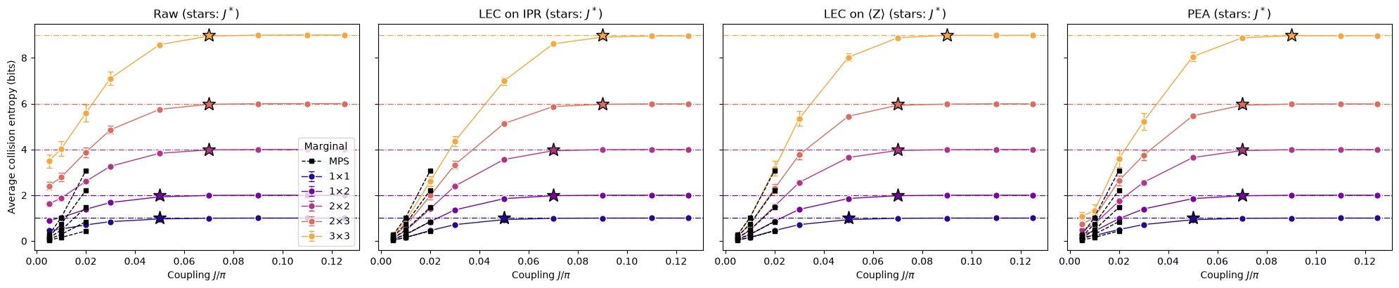
ค่าประมาณทั้งสี่ และ crossover
ฟังก์ชันถัดไปคำนวณค่าประมาณแบบดิบ, LEC บน IPR, LEC บน และ PEA ของ IPR ของ marginal หนึ่งตำแหน่งที่ทุกคัปปลิง และยังประมาณ shot noise ของแต่ละวิธีด้วยการ bootstrap การสุ่ม เซลล์รันฟังก์ชันนี้กับทุกตำแหน่งที่เข้าไปอยู่ในค่าเฉลี่ย ซึ่งใช้เวลาประมาณหนึ่งนาทีครึ่ง
def estimate_iprs(qubits, key):
    # Raw, LEC-on-IPR, LEC-on-<Z>, and PEA IPRs of one marginal position at every coupling,
    # with the shot noise of each from a bootstrap over the randomizations
    n = len(qubits)
    supports = parity_supports(qubits)
    # Parities with shape (noise factors, randomizations, supports), per coupling
    parities = [
        np.stack([parity_expectation_values(b, supports) for b in bits])
        for bits in raw_bits
    ]
    patch_bits = [
        bits[0][:, :, qubits] for bits in raw_bits
    ]  # noise factor 1
    values, errors = lec_estimates(
        patch_bits,
        [p[0] for p in parities],
        references[(calibration_hw, 64)][key],
        calibration_hw,
        n,
    )
    fidelities = np.array([readout_fidelity(s) for s in supports])

    def pea_statistic(p):
        return pea_ipr(p, fidelities, n)

    values["raw"] = [ipr_from_shots(b) for b in patch_bits]
    errors["raw"] = [bootstrap_error(ipr_from_shots, b) for b in patch_bits]
    values["PEA"] = [pea_statistic(p) for p in parities]
    errors["PEA"] = [
        bootstrap_error(pea_statistic, p, axis=1) for p in parities
    ]  # randomizations are axis 1
    return {m: np.array(v) for m, v in values.items()}, {
        m: np.array(e) for m, e in errors.items()
    }

methods = ["LEC on IPR", "LEC on ⟨Z⟩", "PEA"]
method_colors = {
    "LEC on IPR": "#2a78d6",
    "LEC on ⟨Z⟩": "#1baf7a",
    "PEA": "#eb6834",
}
iprs, ipr_errors = {}, {}
for label, patch_list in positions.items():
    for k in kept_placements[label]:
        iprs[label, k], ipr_errors[label, k] = estimate_iprs(
            patch_list[k], f"{label} {k}"
        )
print(f"{len(iprs)} clean marginal positions")
93 clean marginal positions
def crossover_coupling(couplings, entropies, haar, tolerance=0.1):
    # Smallest coupling whose entropy is within tolerance of the random-state value
    for coupling, entropy in zip(couplings, entropies):
        if entropy >= haar - tolerance:
            return coupling
    return None

def reference_ipr(index, chi, key):
    # IPR of the MPS distribution of a marginal
    return float((references[(index, chi)][key] ** 2).sum())

mps_settings = [
    (calibration_hw, 64),
    (1, 128),
    (2, 128),
]  # (coupling index, bond dimension)
panels = ["raw", *methods]

# Average IPR of every shape over its clean placements, then the entropy and the crossover
hw_entropies = {
    method: {} for method in panels
}  # per method and shape: average entropy and its error
crossovers = {method: {} for method in panels}
mps_entropies = {}  # per shape: MPS entropy, averaged over the same placements, at mps_settings
for label, patch_list in positions.items():
    haar = haar_entropy(len(patch_list[0]), num_qubits_hw)
    keys = [(shape, k) for (shape, k) in iprs if shape == label]
    mps_entropies[label] = [
        collision_entropy(
            np.mean([reference_ipr(j, chi, f"{label} {k}") for _, k in keys])
        )
        for j, chi in mps_settings
    ]
    for method in panels:
        ipr, ipr_error = average_ipr(
            [iprs[key][method] for key in keys],
            [ipr_errors[key][method] for key in keys],
        )
        entropy = collision_entropy(ipr)
        hw_entropies[method][label] = (entropy, ipr_error / (ipr * np.log(2)))
        crossovers[method][label] = crossover_coupling(
            couplings_hw, entropy, haar
        )
fig, axes = plt.subplots(
    1, len(panels), figsize=(5 * len(panels), 4.2), sharey=True
)
for (label, patch_list), color in zip(positions.items(), colors):
    haar = haar_entropy(len(patch_list[0]), num_qubits_hw)
    for ax, method in zip(axes, panels):
        entropy, error = hw_entropies[method][label]
        ax.errorbar(
            couplings_hw / np.pi,
            entropy,
            yerr=error,
            fmt="o-",
            color=color,
            mec="white",
            ms=7,
            lw=1,
            capsize=3,
            label=label,
        )
        ax.plot(
            couplings_hw[[j for j, _ in mps_settings]] / np.pi,
            mps_entropies[label],
            "s--",
            color="black",
            ms=4,
            lw=1,
            label="MPS" if label == "3×3" else None,
            zorder=4,
        )
        ax.axhline(haar, color=color, ls="dashdot", lw=0.9)
        if crossovers[method][label]:
            ax.plot(
                crossovers[method][label] / np.pi,
                haar,
                "*",
                ms=14,
                color=color,
                mec="black",
                zorder=3,
            )
for ax, method in zip(axes, panels):
    ax.set_title(f"{'Raw' if method == 'raw' else method} (stars: $J^*$)")
    ax.set_xlabel("Coupling $J/\\pi$")
axes[0].set_ylabel("Average collision entropy (bits)")
axes[0].legend(title="Marginal", loc="lower right")
fig.tight_layout()
plt.show()
สรุป
สิ่งที่ต้องใช้ในการรันการทดลองขนาดนี้:
-
วงจรที่โครงสร้างไม่ขึ้นกับ คอมไพล์ทีละ sublayer ดังนั้นโมเดล noise เดียวจึงใช้ได้กับ sweep ทั้งหมด
-
ตัวประมาณค่าที่ทำงานจาก bitstring: การนับคู่สำหรับ IPR ของ marginal และรูปแบบ Parseval ที่ลบความแปรปรวนจาก parity ยกกำลังสองแต่ละตัว เมื่ออินพุตเป็นค่าคาดหวังที่ผ่าน mitigation แล้ว
-
จุดยึดแบบคลาสสิกที่ราคาถูก: สถานะในอุดมคติที่ ค่าน้อยใช้สอบเทียบ noise และคัปปลิงที่กันไว้ใช้ทดสอบการสอบเทียบ การสอบเทียบ แต่ละตัวแยกกัน แทนที่จะสอบเทียบ IPR ทั้งก้อน คือสิ่งที่ทำให้ marginal ขนาดใหญ่สอดคล้องกัน
-
เครื่องมือของ IBM สำหรับงานหนัก: Samplomatic box และ twirling,
NoiseLearnerV3, dynamical decoupling และงานExecutorหนึ่งงานที่ขยาย noise สำหรับ PEA -
การตรวจสอบคุณภาพข้อมูล ที่ใช้เฉพาะข้อมูล
ขั้นตอนต่อไป หากต้องการทำ mitigation ให้ลึกขึ้น ดูบทแนะนำ probabilistic error amplification และ PEC with shaded lightcones